Download

1 / 23
230 likes | 384 Views
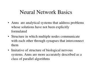
Neural Network Basics. Anns are analytical systems that address problems whose solutions have not been explicitly formulated Structure in which multiple nodes communicate with each other through synapses that interconnect them

E N D
Neural Network Basics • Anns are analytical systems that address problems whose solutions have not been explicitly formulated • Structure in which multiple nodes communicate with each other through synapses that interconnect them • Imitative of structure of biological nervous systems. Anns are more accurately described as a class of parallel algorithms
Knowledge in Anns • Long term knowledge is stored in the networks in the states of the synaptic interconnections – in anns as weights between nodes • Short term knowledge is temporarily stored in the on/off states of the nodes • Both kinds of stored information determine how the network will respond to to inputs
Training of ANNS • Networks are organized by by automated training methods, this simplifies the development of specific applications • There is big advantage in all situations where no clear set of logical rules are given • The inherent fault tolerance of nns is also a big advantage • Nns can also be made to be tolerant against noise in the input : with increased noise the quality of the output only degrades slowly. (Graceful degradation)
Training of Networks • A network will begin with no memories of the input space • A network needs to go through a training phase in which it classifies input vectors
One of the major advantages of nns is their ability to generalize. This means that a trained net could classify data from the same class as the learning data that it has never seen before • Training set – used to train the net • Validation set – used to determine the the performance of the net on patterns not trained during learning phase • A test set for finally checking the over all performance of a NN
Mcculloch Pitts Model • Acts a feature detector • N inputs • N weights • M outputs • Threshold θ
Mcculloch Pitts Model • Input is modulated by weighting the value of the connection • Input is then integrated by the unit to produce the stimulation signal to the unit • This becomes the activation • If activation if >= θ the neuron fires • Inhibitory input is absolute in keeping a neuron off
Mcculloch Pitts Model • The mcculloch pitts model is severely limited • Can only categorize linearly separable domains • No training regime
Rosenblatt’s Perceptron • Single layer network • Again can categorize patterns • However a training algorithm exist to adjust weights within the network which causes the network to ‘learn’ • Hebbian learning algorithm used
Hebbian Learning • Donald hebb proposed a learning theory • If a neuron X in a nervous system repeatedly stimulates a second neuron, Y to fire, then the pathways from X to Y becomes increasingly efficient in conveying that stimulus • The perceptron is essentially mcculloch pitt’s model with hebbian training model
Problem With the Perceptron • Minksy & papert proved the perceptron couldn’t categorize a problem as simple as the XOR problem
Introduction of a Hidden Layer • The hidden layer solves the issue of linear separability • This introduces the idea of a multi-layer network, the multi-perceptron is born
The Dawn of New Networks • Back-propagation • Hopfield • Kohonen SOM – self organizing maps
The Back-propagation Algorithm • Essentially a multi-layer perceptron with • A different threshold function • A more robust capable learning rule • Backprop acts as a classifier/predictor eg. Loan evaluation • A trained network is guaranteed to find relationships between input and output presented to it
Neural networks are universal approximators • Backprop has been shown to always find the right model it will always converge
Training a Back Propagation Network • An input pattern is propagated forward in the net until activation reaches the output layer • The output at the output layer is compared with the teaching input • The error j (if there is one) is propagated back through the network from the output through the hidden layers weights are adjusted so that all those nodes that contribute to the error are adjusted
Backprop • In online learning the change in weights are applied to the network after each training pattern after each forward and back pass • In offline or batch learning the weight changes are cumulated for all patterns in the input set after one full cycle (epoch) through the training pattern file • In the back propagation algorithm online training is usually faster than batch training especially in the case of large training sets with many similar examples
Limitations of Neural Networks • Scalability • Neural networks can become unstable when applied to larger problems
A simple example - OR (single layer see diagrams below) We want a network to be able to respond to learn the OR input pattern Input Output 0 0 0 0 1 1 1 0 1 1 1 1 The network has 2 inputs, and one output. All are binary. The output is determined by 1 if W0 *I0 + W1 * I1 > 0 0 if W0 *I0 + W1 * I1 <= 0 We want it to learn simple OR: output a 1 if either I0 or I1 is 1.
Single layer Input 1 output Input 2
Inside the neuronstage 1 W1 * input1 Input 1 output = Activation + Input 2 W2 W2 * input2
Inside the neuronstage 2 If activation (a) >= threshold () output = 1 else output =0 Input 1 output Input 2
Neuron fundamentalsactivation a = wixithreshold = output = 1 if a >= thresholdoutput = 0 if a <threshold-1 > wi < 1