Download
1 / 71
710 likes | 815 Views
Robust Feature-Based Registration of Remotely Sensed Data. Nathan S. Netanyahu Dept. of Computer Science, Bar-Ilan University and Center for Automation Research, University of Maryland Collaborators: Jacqueline Le Moigne NASA / Goddard Space Flight Center

E N D
Robust Feature-Based Registration of Remotely Sensed Data Nathan S. Netanyahu Dept. of Computer Science, Bar-Ilan University and Center for Automation Research, University of Maryland Collaborators: Jacqueline Le Moigne NASA / Goddard Space Flight Center David M. Mount University of Maryland Arlene A. Cole-Rhodes, Kisha L. Johnson Morgan State University, Maryland Roger D. EastmanLoyola College of Maryland Ardeshir Goshtasby Wright State University, Ohio Jeffrey G. Masek, Jeffrey Morisette NASA / Goddard Space Flight Center Antonio Plaza University of Extremadura, Spain San Ratanasanya King Mongkut’s University, Thailand Harold Stone NEC Research Institute (Ret.) Ilya Zavorin CACI International, Maryland Shirley Barda, Boris Sherman Applied Materials, Inc., Israel Yair Kapach Bar-Ilan University
What is Image Registration / Alignment / Matching? The above image over Colorado Springs is rotated and shifted with respect to the left image.
Definition and Motivation • Task of bringing together two or more digital images into precise alignment for analysis and comparison • A crucial, fundamental step in image analysis tasks, where final information is obtained by the combination / integration of multiple data sources.
Motivation / Applications • Computer Vision (target localization, quality control, stereo matching) • Medical Imaging (combining CT and MRI data, tumor growth monitoring, treatment verification) • Remote Sensing (classification, environmental monitoring, change detection, image mosaicing, weather forecasting, integration into GIS)
Literature of Automatic Image Registration • Books: • Medical Image Registration, J. Hajnal, D.J. Hawkes, and D. Hill (Eds.), CRC 2001 • Numerical Methods for Image Registration, J. Modersitzki, Oxford University Press 2004 • 2-D and 3-D Image Registration, A. Goshtasby, Wiley 2005 • Image Registration for Remote Sensing, J. LeMoigne, N.S. Netanyahu, and R.D. Eastman (Eds.), Cambridge University Press 2011 • Surveys: • A Survey of Image Registration Techniques, ACM Comp. Surveys, L.G. Brown, 1992 • Registration Techniques for Multisensor Remotely Sensed Imagery, PE&RS, L.M.G. Fonseca and B.S. Manjunath, 1996 • A Survey of Medical Image Registration, Medical Image Analysis, J.B.A. Maintz and M.A. Viergever, 1998 • Image Registration Methods: A Survey, Image and Vision Computing, B. Zitová and J. Flusser, 2003 • Mutual-Information-Based Registration of Medical Images: A Survey, IEEE-TMI, J. Pluim, J.B.A. Maintz, and M.A. Viergever, 2003
Application Examples • Change Detection 2000 1975 Satellite images of Dead Sea, United Nations Environment Programme (UNEP) website
Change Detection (cont’d) IKONOS images of Iran’s Bushehr nuclear plant, GlobalSecurity.org
Change Detection (cont’d) Satellite imagery of Sendai Airport before and after the 2011 earthquake
Automatic Image Registration for Remote Sensing • Sensor webs, constellation, and exploration • Selected NASA Earth science missions • IR challenges in context of remote sensing
Sensor Webs, Constellation, and Exploration Planning and Scheduling Automatic Multiple Source Integration Satellite/Orbiter, and In-Situ Data Intelligent Navigation and Decision Making
MODIS Satellite System From the NASA MODIS website
Landsat-7 Satellite System New Orleans, before and after Katrina 2005 (from the USGS Landsat website)
Image Registration in the Context of Remote Sensing • Navigation or model-based systematic correction • Orbital, attitude, platform/sensor geometric relationship, sensor characteristics, Earth model, etc. • Image Registrationor feature-based precision correction • Navigation within a few pixels accuracy • Image registration using selected features (or control points) to refine geolocation accuracy • Two common approaches: (1) Image registration as post processing (taken here) (2) Navigation and image registration in closed loop
Challenges in Registration of Remotely Sensed Imagery • Multisource data • Multitemporal data • Various spatial resolutions • Various spectral resolutions • Subpixel accuracy • 1 pixel misregistration ≥ 50% error in NDVI classification • Computational efficiency • Fast procedures for very large datasets • Accuracy assessment • Synthetic data • Ground truth (manual registration?) • Consistency (circular registrations) studies
Fusion of Multitemporal Images Improvement of NDVI classification accuracy due to fusion of multitemporal SAR and Landsat TM over farmland in The Netherlands (source: The Remote Sensing Tutorial by N.M. Short, Sr.)
Integration of Multiresolution Sensors Registration of Landsat ETM+ and IKONOS images over coastal VA and agricultural Konza site (source: J. LeMoigne et al., IGARSS 2003)
What is the “Big Deal” about IR? By matching control points, e.g., corners, high-curvature points. How do humans solve this? Zitová and Flusser, IVC 2003
Automatic Image Registration Components 0. Preprocessing • Image enhancement, cloud detection, region of interest masking 1. Feature extraction (control points) • Corners, edges, wavelet coefficients, segments, regions, contours 2. Feature matching • Spatial transformation (a priori knowledge) • Similarity metric (correlation, mutual information, Hausdorff distance, discrete Gaussian mismatch) • Search strategy (global vs. local, multiresolution, optimization) 3. Resampling I2 Tp I1
Example of Image Registration Steps Feature extraction Resampling Registered images after transformation Zitová and Flusser, IVC 2003 Feature matching
Step 1: Feature Extraction Gray levels BPF wavelet coefficients Binary feature map Top 10% of wavelet coefficients (due to Simoncelli) of Landsat image over Washington, D.C. (source: N.S. Netanyahu, J. LeMoigne, and J.G. Masek, IEEE-TGRS, 2004)
Step 1: Feature Extraction (cont’d) Image features (extracted from two overlapping scenes over D.C.) to be matched
Step 2: Feature Matching / Transformations • Given a reference image, I1(x, y), and a sensed image I2(x, y),find the mapping (Tp, g) which “best” transforms I1 intoI2, i.e., where Tp denotes spatial mapping and g denotes radiometric mapping. • Spatial transformations: Translation, rigid, affine, projective, perspective, polynomial • Radiometric transformations (resampling): Nearest neighbor, bilinear, cubic convolution, spline
Step 2: Transformations (cont’d) Objective: Find parameters of a transformation Tp (consisting of a translation, a rotation, and an isometric scale) that maximize similarity measure.
Step 2: Similarity Measures (cont’d) • L2-norm: Minimize sum of squared errors over overlapping subimage • Normalized cross correlation (NCC): Maximize normalized correlation between the images
Step 2: Similarity Measures (cont’d) • Mutual information (MI): Maximize the degree of dependence between the images or using histograms, maximize
Step 2: Similarity Measures (cont’d), An Example MI vs. L2-norm and NCC applied to Landsat-5 images (source: H. Chen, P.K. Varshney, and M.K. Arora, IEEE-TGRS, 2003)
Step 2: Similarity Measures (cont’d):An MI Example Source: A.A. Cole-Rhodes et al., IEEE-TIP, 2003
Step 2: Similarity Measures (cont’d) • (Partial) Hausdorff distance (PHD): where
Step 2: Similarity Measures (cont’d):A PHD Example PHD-based matching of Landsat images over D.C.(source: N.S. Netanyahu, J. LeMoigne, and J.G. Masek, IEEE-TGRS, 2004)
Step 2: Similarity Measure (cont’d) • Discrete Gaussian mismatch (DGM) distance: where denotes the weight of point a, and is the similarity measure ranging between 0 and 1
Step 2: Feature Matching / Search Strategy • Exhaustive search • Fast Fourier transform (FFT) • Optimization (e.g., gradient descent; Thévenaz, Ruttimann, and Unser (TRU), 1998; Spall, 1992) • Robust feature matching (e.g., efficient subdivision and pruning of transformation space; Huttenlocher et al., 1993, Mount et al., 1999, 2011)
Search Strategy: Geometric Branch and Bound • Space of affine transformations: 6-D space • Subdivide: Quadtree or kd-tree. Each cell Trepresents a set of transformations;T is active if it may contain ; o/w, it is killed • Uncertainty regions (UR’s): Rectangular approximation to the possible images for all • Bounds: Compute upper bound (on optimum similarity) by sampling a transformation and lower bound by computing nearest neighbors to each UR • Prune: If lower bound exceeds best upper bound, then kill the cell; o/w, split it
Branch and Bound (cont’d) Illustration of uncertainty regions
Algorithmic Outline of B & B (Sketch) • For all active cells do • Compute upper bound on similarity metric • For each active compute a lower bound on the similarity measure (can be done using a variant of efficient NN-searching) • Prune search space, i.e., discard if lower bound exceeds best (upper bound) seen thus far • O/w, split (e.g., along “longest dimension”) and enqueue in queue of active cells • If termination condition met, e.g., empty or , then report transformation and exit; o/w, goto 1)
Extended B & B Framework • Approximate algorithm applies to both PHD and DGM • Upper bound variants: • Pure • Bounded alignment (BA) • Bounded least squares alignment (BLSA) • Priority strategies for picking next cell • Maximum uncertainty (MaxUN) • Minimum upeer bound (MinUB) • Minimum lower bound (MinLB)
Upper Bound Variants • Pure: • Cell midpoint is candidate transformation • Bounded alignment (BA): • Apply Monte Carlo sampling, i.e., sample a small number of point pairs, provided that UR of a point contains only one point from the other set • For each point pair compute a transformation • Return transformation whose distance is smallest • Bounded least squares alignment (BLSA): • Apply iterative closest pair; first compute transformation that aligns centroids, then compute scale (that aligns spatial variances), and then compute rotation which mininmizes sum of squared distances
Search Priorities • Maximum uncertainty (MaxUN): • Next active cell with largest average diameter of its URs • Minimum upper bound (MinUB): • Next active cell with smallest upper bound • Minimum lower bound (MinLB): • Next active cell with smallest lower bound
Dataset Features Superimposed VA Cascades Konza
Experimental Results forVA, Cascades, and Konza Sites (Exp.1) VA Cascades Konza
Experimental Results (cont’d) forVA, Cascades, and Konza Sites (Exp. 2) VA Cascades Konza
Performance Results on Tested Sites • Tested running time and transformation distance • MinLB demonstrated best performance • DGM (with certain , e.g., ) outperforms PHD; see in particular VA dataset (IR-IN) • Comparable performance across same image pairings (e.g., Cascades and Konza) • BA was almost always fastest but had highest degree of variation in accuracy • In general, demonstrated the algorithm’s efficacy for many additional datasets, including multisensor images covering various spectral bands
Computational Efficiency • Efficient search strategy (e.g., B & B variants) • Hierarchical, pyramid-like approach • Extraction of corresponding regions of interest(ROI)
Computational Efficiency (cont’d):An Example of a Pyramid-Like Approach 0 32 x 32 1 64 x 64 2 128 x 128 3 256 x 256
Hierarchical IR ExampleUsing Partial Hausdorff Distance 64 x 64 128 x 128 256 x 256
Image Registration Subsystem Based on a Chip Database input scene UTM of 4 scene corners known from systematic correction (1) Find chips that correspond to the incoming scene (2) For each chip, extract window from scene, using UTM of: - 4 approx. scene corners - 4 correct chip corners (3) Register each (chip-window) pair and record pairs of registered chip corners (4) Compute global transformation from multiple local registrations (5) Compute correct UTM of 4 scene corners of input scene Landmark chip database correct UTM of 4 chip corners