Download
1 / 29
290 likes | 413 Views
ECEN4503 Random Signals Lecture #24 10 March 2014 Dr. George Scheets. Read 8.1 Problems 7.1 - 7.3, 7.5 (1 st & 2 nd Edition) Next Quiz on 28 March Exam #1 Results Hi = 94, Low = 36, Average = 69.53, σ = 13.41 A > 88, B > 78, C > 64, D > 51.

E N D
ECEN4503 Random SignalsLecture #24 10 March 2014Dr. George Scheets Read 8.1 Problems 7.1 - 7.3, 7.5 (1st & 2nd Edition) Next Quizon 28 March Exam #1 ResultsHi = 94, Low = 36, Average = 69.53, σ = 13.41A > 88, B > 78, C > 64, D > 51
ECEN4503 Random SignalsLecture #25 12 March 2014Dr. George Scheets • Read 8.3 & 8.4 • Problems 5.5, 5.7, 5.20 (1st Edition) • Problems 5.10, 5.21, 5.49 (2nd Edition)
Random Number Generator • Uniform over [0,1] • TheoreticalE[X] = 0.5σX = (1/12)0.5 = 0.2887 • ActualE[X] = 0.5003σX = 0.2898
Random Number Generator • Addition of 2 S.I. Uniform Random Numbers → Triangular PDF • Each Uniform over [0,1] • TheoreticalE[X] = 1.0σX = (2/12)0.5 = 0.4082 • ActualE[X] = 1.008σX = 0.4114
Random Number Generator • Addition of 3 S.I. Uniform Random Numbers → PDF starting to look Bell Shaped • Each Uniform over [0,1] • TheoreticalE[X] = 1.5σX = (3/12)0.5 = 0.5 • ActualE[X] = 1.500σX = 0.5015
RXY for age & weight X = Age Y = Weight RXY ≡ E[XY] = 4322 (85 data points)
RXY for age & middle finger length X = Age Y = Finger Length (cm) RXY ≡ E[XY] = 194.2 (54 data points)
Cov(X,Y) for age & weight X = Age Y = Weight RXY ≡ E[XY] = 4322 E[Age] = 23.12 E[Weight] = 186.4 E[X]E[Y] = 4309 Cov(X,Y) = 13.07 (85 data points)
Cov(X,Y) for age & middle finger length X = Age Y = Finger Length RXY ≡ E[XY] = 194.2 E[Age] = 22.87 E[Length] = 8.487 E[X]E[Y] = 194.1 Cov(X,Y) = 0.05822 (54 data points)
Age & Weight Correlation Coefficient ρ X = Age Y = Weight Cov(X,Y) = 13.07 σAge = 1.971 years σWeight = 39.42 ρ = 0.1682 (81 data points)
Age & Weight Correlation Coefficient ρ X = Age Y = Weight Cov(X,Y) = 13.07 σAge = 1.971 years σWeight = 39.42 ρ = 0.1682 (85 data points)
Age & middle finger length Correlation Coefficient ρ X = Age Y = Finger Length Cov(X,Y) = 0.05822 σAge = 2.218 years σLength = 0.5746 ρ = 0.04568 (54 data points)
SI versus Correlation • ρ ≡ Correlation CoefficientAllows head-to-head comparisons (Values normalized) ≡ E[XY] – E[X]E[Y]σXσY = 0? → We say R.V.'s are Uncorrelated = 0 < ρ < 1 → X & Y tend to behave similarly = -1 < ρ < 0 → X & Y tend to behave dissimilarly • X & Y are S.I.? → ρ = 0 → X & Y are Uncorrelated • X & Y uncorrelated? → E[XY] = E[X]E[Y] • Example Y = X2; fX(x) symmetrical about 0 • Here X & Y are dependent, but uncorrelated • See Quiz 6, 2012, problem 1e
Two sample functions of bit streams. 1.25 1.25 1 1 x x i i 0 0 1 1 1 1 0 50 100 150 200 250 300 350 400 0 20 40 60 80 100 0 i 400 0 i 100
Random Bit Stream. Each bit S.I. of others.P(+1 volt) = P(-1 volt) = 0.5 1.25 1 x i 0 1 1 0 20 40 60 80 100 0 i 100 fX(x) 1/2 -1 x volts +1
Bit Stream. Average burst length of 20 bits.P(+1 volt) = P(-1 volt) = 0.5 1.25 1 x i 0 1 1 0 50 100 150 200 250 300 350 400 0 i 400 Voltage Distribution of this signal & previous are the same, but time domain behavior different. fX(x) 1/2 -1 x volts +1
Review of PDF's & Histograms Probability Density Functions (PDF's), of which a Histogram is an estimate of shape, frequently (but not always!) deal with the voltage likelihoods Volts Time
Discrete Time Noise Waveform255 point, 0 mean, 1 wattUniformly Distributed Voltages Volts 0 Time
15 Bin Histogram(255 points of Uniform Noise) Bin Count 0 Volts
15 Bin Histogram(2500 points of Uniform Noise) Bin Count When bin count range is from zero to max value, a histogram of a uniform PDF source will tend to look flatter as the number of sample points increases. 200 0 0 Volts
15 Bin Histogram(2500 points of Uniform Noise) Bin Count But there will still be variation if you zoom in. 200 140 0 Volts
15 Bin Histogram(25,000 points of Uniform Noise) 2,000 Bin Count 0 0 Volts
Bin Count Volts Time Volts The histogram is telling us which voltages were most likely in this experiment. A histogram is an estimate of the shape of the underlying PDF. 0
Discrete Time Noise Waveform255 point, 0 mean, 1 wattExponentially Distributed Voltages Volts 0 Time
15 bin Histogram(255 points of Exponential Noise) Bin Count 0 Volts
Discrete Time Noise Waveform255 point, 0 mean, 1 wattGaussian Distributed Voltages Volts 0 Time
15 bin Histogram(255 points of Gaussian Noise) Bin Count 0 Volts
15 bin Histogram(2500 points of Gaussian Noise) Bin Count 400 0 Volts