Download
1 / 27
300 likes | 503 Views
Impossibility of Distributed Consensus with One Faulty Process. Michael J. Fischer Nancy A. Lynch Michael S. Paterson. Presented by: Oren D. Rubin. Agenda:. Motivation The Consensus Problem Goal Assumptions Terminology Main. Motivation. General 2 ’ s army.

E N D
Impossibility of Distributed Consensus with One Faulty Process Michael J. Fischer Nancy A. Lynch Michael S. Paterson Presented by: Oren D. Rubin
Agenda: • Motivation • The Consensus Problem • Goal • Assumptions • Terminology • Main
Motivation General 2’s army • 4 allied armies, each one led by a general, besiege a castle. • To seize castle, all fourmust attack together, otherwise armies defeats General 1’s army General 3’s army • Communications by messengers, reliable, but take unbounded time… • A Generals may get killed !! (and never be replaced) General 4’s army
Motivation… Transaction commit – all data managers must make the same decision in order to preserve the consistency of the database. Can I commit? Yes!! No!!
The Consensus Problem • There is a set of distributed processes with initial values {0,1} • This strengthen the impossibility result and simplifies the discussion. • They must all decide on the same value {0,1}, based on their initial states. • There must be some initial state of the process set for which the reached decision is 0 and another for which it is 1. • To avoid trivial consensus protocols (which always result in the same decision) • Some “non-faulty” processes eventually decide on some value and this decision is irrevocable
Goal No completely asynchronous consensus protocol can tolerate even a single unannounced process death (no Byzantine failures).
Assumptions Processing is completely asynchronous • Reliable, includes “atomic broadcast” (virtual synchrony), could be out of order. • No assumptions about the relative speeds of processes. • Unknown delay time in message delivery. • No access to synchronized clocks (no time - outs). • No ability to detect the death of a process.
Terminology • System Model- message passing based. • message is apair of (p, m) : destination processand message value • N (>1) processes • The message system • Holds a message buffer • Unbounded. • Supports operations • Send(p,m) - places (p,m) in message buffer. • Receive(p) – extract a message (p,m) from the message buffer (m is delivered) or return “null” (finite number of times).
Terminology ... • Process–automaton, finite or infinite states (deterministic). Each process p comprises an internal state • Input register Xp -fixed initial value. • output register Yp - initialed with ‘b’ (blank), fixed after rewritten. • Internal storage - unbounded, fixed initial value. Performs atomic steps (A.K.A. events) composed of - • Receive a message (could be “null”). • Changes state (depending on message received). • Sends finite set of messages to other processes • Configuration– system’s global state, comprises all processes’ internal states and the message buffer • Initial configuration: initial states for all processes and message buffer is empty. • A step takes one configuration to another (completely determined by (p,m) ).
Terminology ... • Event:(on process p) e = (p,m) : process p performs an atomic step. • Message m delivered to p. • Triggers state transition in p. • Finite number of message sent by p (p, “null”) can always be applied on a configuration • Event e applicable to configuration C:if e message buffer or e = (p,“null”). • e(C): resulting configuration after applying event e on configuration C: • Process p has a new internal state (the one resulted from message being delivered). • All other processes’ states unchanged. • Message buffer changed (e removed, process's messages added, if any).
Terminology ... • Schedule (run):finite/infinite sequence of events that can be applied on a configuration C0. • Events are applicable to configuration C0 • S = e1e2e3…ei… • S(C0) is the configuration resulted a finite run. • Reachable configuration C’ from C:If a finite run S exists such that S(C0) = C’. • If C0 is an initial configuration then C’ is said to beaccessible. C0 C1 C2 Ci e1 e2 e3 … ei ei+1
Terminology ... • Non-faulty process in a run: a process that take infinitely number of steps on that run, Faulty otherwise. • Admissible run: a run with one faulty member at most and all messages to non-faulty members will be delivered eventually. • Decision value of a configuration C: a set of all processes’ non-blank Yp values (their decision states). • Only 4 Decision values possible: {}, {0}, {1}, {0,1} • Deciding run: some process reaches a decision states during the run i.e. a process sets his Yp value (to either 0 or 1). • Partially correct protocol: • All accessible configuration don’t have more than one decision value • There exists two accessible configurations G and H S.T. their decision values are {0} and {1} correspondingly • Totally correct protocol: • Partially correct. • Every admissible run is a deciding ones.
Terminology ...Valence of configuration C • C is 0-valent: for every schedule S applicable to C, if process p decides on a value v in S(C) then v=0. I.e. S(C) Decision values is either {} or {0} C may be 0-valent although no process has decided {0} yet!! • C is 1-valent: similar definition. • C is univalent: C is either 0-valent or 1-valent I.e. fate of decision definitive!! • C is bivalent: exists schedules S0 and S1, applicable to C, such that: • S0(C) is 0-valent • S1(C) is 1-valent I.e. both decisions are still possible!!
Terminology ... Valence of configuration C 0-valent Configuration p7.Yp = 0 e’5 0-valent configuration 0-valent configuration 0-valent Configuration p1.Yp = 0 e’’ … e’ bivalent configuration e e’’’ bivalent configuration 1-valent configuration e’’’’ 1-valent Configuration p7.Yp = 1 …
Main Event Commutatively: Let C be any configuration and e, e’ be any events applicable to C occurring to differentprocesses. Then e( e’(C) )= e’( e(C) ) C0 e’ e C1 C2 e e’ C3
Main • Schedule Commutatively: Let C be any configuration and S, S’ be any events applicable to C occurring to differentprocesses. Then • S( S’(C) )= S’( S(C) ) C0 S’ S C1 C2 S S’ C3
Main • Event Commutatively Proof: • Internal states of the process involved are mutual excluded. • The message buffer is a set. • Schedule Commutatively Proof: • e1e2e3…ei…en e’1e’2e’3…e’i…e’m • e1e2e3…ei…e’1 ene’2e’3…e’i…e’m • e’1e1e2e3…ei…en e’2e’3…e’i…e’m • e’1e’2e’3…e’i…e’m e1e2e3…ei…en S S’ S’ S
Main • Lemma 1: Every Totally correct protocol has an initial configuration C that is bivalent • There is an initial configuration C0 that is 0-valent • There is an initial configuration C1 that is 1-valent • Let’s assume the contrary, that all configuration are univalent (since the protocol is partial correct). • Adjacent configuration: 2 configurations are adjacent is they differ in only one process’s (process pi) Xp value. There must exist adjacent configurations C0, C1 S.T. C0 is 0-valent and C1 is 1-valent (next slide). Take any admissible deciding run (with schedule S) where process pi takes no steps (one faulty process allowed). S can be applied to both C0 and C1 and they both will reach the same decision value (since nothing changes except pi’s Xp value which is untouched). decision value=1 C0 is bivalent. decision value=0 C1 is bivalent. Contradiction!!!
Main Not necessary The 1-valent adjacent P1 Xp=1 Xp=1 Xp=0 Xp=1 Xp=1 Xp=1 Xp=1 P0 Xp=0 Xp=0 Xp=1 Pi Xp=1 Xp=1 processes Xp=0 Xp=0 Xp=0 Xp=0 Xp=0 Xp=0 Xp=1 Pn Xp=0 1-valent 0-valent
Main • Lemma 2:Let C be any bivalent configuration, and e be any event applicable to C. There exists a finite schedule S applicable to C that does not contain e, such that e( S (C) ) is also bivalent. F = { S(C) : S finite schedule applicable to C that does not contain e} D = {e(C’) : C’ F} Need to show that D contains a bivalent configuration. D configurations Bivalent e e e e e e e e e F configurations
Main Assume the contrary, D doesn’t have a bivalent configuration • Neighbors configuration: configuration C0 and C1 are neighbors if one resulted from the other in one step e’ = (p’,m’) There exists neighbors C0, C1 S.T. C1=e’(C0) or C0=e’(C1) And that D1=e(D0), D0=e(D1) are 1-valent and 0-valent correspondingly (next slide)
Main • Key: Though each run can be infinite, in finite number of step the run is decided Algorithm to findingC0, C1 • Start with a bivalent configuration • If there exists an event e’’ that leads to bivalent configuration then go to b with e(C). else (must be eventually because protocol is totally correct) all events lead to univalent configuration including e (which lead to a 0-valent or a 1-valent configuration) but there must exist another event e’’’ which leads to the other-valent (since we reached a bivalent configuration) 0-valent Configuration p7.Yp = 0 e’5 0-valent configuration 0-valent configuration e’’ e’’’’ … 0-valent Configuration p1.Yp = 0 e C0 C1 bivalent configuration 1-valent configuration e’’’ bivalent configuration e’ … 1-valent Configuration p7.Yp = 1
Main … (proof continued) • Without loss of generality C1=e’(C0) D0 D1 F configurations e e C1 C0 e’ D configurations
Main • Case 1: p not equals to p’ • By the commutatively property D1 is 0-valent and 1-valent, Contradiction!! D0 D1 e’ F configurations e e C1 C0 e’ D configurations
Main • Case 1: p equals to p’ • Be S the schedule of a finite deciding run in which process p takes no steps (S is applicable to D1 and D0 due to commutatively) S(C0)=A by commutatively e(A)=E0 = S( e(C0) ) which is 0-valent configuration Also by commutatively e(A)=E1 = S( e’( e(C0) ) ) which is 1-valent configuration But since S is a deciding run A must be a univalent configuration and applying events on it only lead to univalent configuration Contradiction !! E0 0-valent S e D0 A e’ e 1-valent e S E0 S C1 C0 D1 e e’
Main… finally • The last 2 contradictions proved that D contains a bivalent configuration. • The idea: postpone the event that leads to a univalent configuration by that delaying the decision. • The algorithm: a. Execution begins with the bivalent configuration C0 which is promised. b. we order the messages in the message buffer, according to the time they were sent, earliest first. c. We go over the processes in a round robin fashion (infinitely), for each process: • Let m be the first message in the message buffer destined to the process in the head of the queue or “null” • By lemma 2 there exists a bivalent configuration C’ S.T. C’ is reachable from C by a schedule S in which (p,m) is the last step applied. • We apply S. since all messages are delivered this infinite run is admissible.