Download
1 / 22
220 likes | 391 Views
Reinforcement Learning: Learning algorithms. Yishay Mansour Tel-Aviv University. Outline . Last week Goal of Reinforcement Learning Mathematical Model (MDP) Planning Value iteration Policy iteration This week: Learning Algorithms Model based Model Free. Planning - Basic Problems.

E N D
Reinforcement Learning:Learning algorithms Yishay Mansour Tel-Aviv University
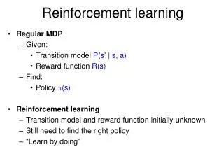
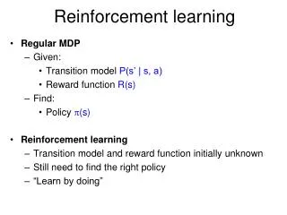
Outline • Last week • Goal of Reinforcement Learning • Mathematical Model (MDP) • Planning • Value iteration • Policy iteration • This week: Learning Algorithms • Model based • Model Free
Planning - Basic Problems. Given a complete MDP model. Policy evaluation - Given a policy p, estimate its return. Optimal control - Find an optimal policy p*(maximizes the return from any start state).
Planning - Value Functions Vp(s)The expected value starting at state s followingp. Qp(s,a)The expected value starting at state s with action a and then followingp. V*(s) and Q*(s,a) are define usingan optimal policy p*. V*(s) = maxpVp(s)
Algorithms - optimal control CLAIM: A policy p is optimal if and only if at each state s: Vp(s) = MAXa{Qp(s,a)} (Bellman Eq.) The greedy policy with respect to Qp(s,a) is p(s) = argmaxa{Qp(s,a) }
MDP - computing optimal policy 1. Linear Programming 2. Value Iteration method. 3. Policy Iteration method.
Planning versus Learning Tightly coupled in Reinforcement Learning Goal: maximize return while learning.
Example - Elevator Control Learning (alone): Model the arrival model well. Planning (alone) : Given arrival model build schedule Real objective: Construct a schedule while updating model
Learning Algorithms Given access only to actions perform: 1. policy evaluation. 2. control - find optimal policy. Two approaches: 1. Model based (Dynamic Programming). 2. Model free (Q-Learning).
Learning - Model Based Estimate the model from the observation. (Both transition probability and rewards.) Use the estimated model as the true model, and find optimal policy. If we have a “good” estimated model, we should have a “good” estimation.
Learning - Model Based: off policy • Let the policy run for a “long” time. • what is “long” ?! • Build an “observed model”: • Transition probabilities • Rewards • Use the “observed model” to estimate value of the policy.
Learning - Model Basedsample size Sample size (optimal policy): Naive: O(|S|2 |A| log (|S| |A|) ) samples. (approximates each transition d(s,a,s’) well.) Better: O(|S| |A| log (|S| |A|) ) samples. (Sufficient to approximate optimal policy.) [KS, NIPS’98]
Learning - Model Based: on policy • The learner has control over the action. • The immediate goal is to lean a model • As before: • Build an “observed model”: • Transition probabilities and Rewards • Use the “observed model” to estimate value of the policy. • Accelerating the learning: • How to reach “new” places ?!
Learning - Model Based: on policy Relatively unknown nodes Well sampled nodes
Learning: Policy improvement • Assume that we can perform: • Given a policy p, • Compute V and Q functions of p • Can run policy improvement: • p = Greedy (Q) • Process converges if estimations are accurate.
Learning: Monte Carlo Methods • Assume we can run in episodes • Terminating MDP • Discounted return • Simplest: sample the return of state s: • Wait to reach state s, • Compute the return from s, • Average all the returns.
Learning: Monte Carlo Methods • First visit: • For each state in the episode, • Compute the return from first occurrence • Average the returns • Every visit: • Might be biased! • Computing optimal policy: • Run policy iteration.
Learning - Model FreePolicy evaluation: TD(0) An online view: At state st we performed action at, received reward rtand moved to state st+1. Our “estimation error” isAt =rt+gV(st+1)-V(st), The update: Vt +1(st) = Vt(st ) + a At Note that for the correct value function we have: E[r+gV(s’)-V(s)] =0
Learning - Model FreeOptimal Control: off-policy Learn online the Q function. Qt+1 (st ,at ) = Qt (st ,at )+ a [ rt+g Vt (st+1) - Qt (st ,at )] OFF POLICY: Q-Learning Any underlying policy selects actions. Assumes every state action performed infinitely often Learning rate dependency. Convergence in the limit: GUARANTEED [DW,JJS,S,TS]
Learning - Model FreeOptimal Control: on-policy Learn online the Q function. Qt+1 (st ,at ) = Qt (st ,at )+ a [ rt+g Qt (st+1,at+1) - Qt (st ,at )] ON-Policy:SARSA at+1 the e-greedy policy for Qt. The policy selects the action! Need to balance exploration and exploitation. Convergence in the limit: GUARANTEED [DW,JJS,S,TS]
Learning - Model FreePolicy evaluation: TD() Again: At state st we performed action at, received reward rtand moved to state st+1. Our “estimation error” A=rt+gV(st+1)-V(st), Update every state s: Vt +1(s) = Vt(s) + a A e(s) Update of e(s) : When visiting s: incremented by 1: e(s) = e(s)+1 For all s: decremented by g every step: e(s) = g e(s)
Summary Markov Decision Process: Mathematical Model. Planning Algorithms. Learning Algorithms: Model Based Monte Carlo TD(0) Q-Learning SARSA TD()