Download
1 / 87
900 likes | 1.12k Views
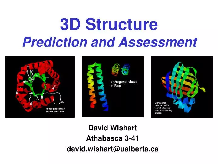
3D Structure Prediction and Assessment. David Wishart Athabasca 3-41 david.wishart@ualberta.ca. Outline & Objectives*. Become familiar with the Protein Universe and the Protein Structure Initiative Learn principles of how to do homology (comparative) modelling of 3D protein structures

E N D
3D StructurePrediction and Assessment David Wishart Athabasca 3-41 david.wishart@ualberta.ca
Outline & Objectives* • Become familiar with the Protein Universe and the Protein Structure Initiative • Learn principles of how to do homology (comparative) modelling of 3D protein structures • Learn how to do homology modelling on the Web • Learn how to assess 3D structures (modelled and experimental)
Structural Proteomics: The Motivation 120,000,000 100,000,000 80,000,000 60,000,000 40,000,000 20,000,000 0 600000 500000 400000 300000 200000 100000 0 Sequences Structures
Protein Structure Initiative* • Organize all known protein sequences into sequence families • Select family representatives as targets • Solve the 3D structures of these targets by X-ray or NMR • Build models for the remaining proteins via comparative (homology) modeling
Protein Structure Initiative* • Organize and recruit interested structural biologists and structure biology centres from around the world • Coordinate target selection • Develop new kinds of high throughput techniques • Solve, solve, solve, solve….
The Protein Fold Universe 500? 2000? 10000? How Big Is It??? 8 ? Human Genome Codes for ~21,000 Proteins
Structure Deposition Rate • Growth has been exponential for the past 10 years • Approximately 8000 new structures being added each year
Protein Structure Initiative • 25,000 proteins • 10,000 subset • 30% ID or • 30 seq • Solve by 2010 • $20,000/Structure 30 seq
Comparative (Homology) Modelling ACDEFGHIKLMNPQRST--FGHQWERT-----TYREWYEGHADS ASDEYAHLRILDPQRSTVAYAYE--KSFAPPGSFKWEYEAHADS MCDEYAHIRLMNPERSTVAGGHQWERT----GSFKEWYAAHADD
Homology Modelling* • Based on the observation that “Similar sequences exhibit similar structures” • Known structure is used as a template to model an unknown (but likely similar) structure with known sequence • First applied in late 1970’s using early computer imaging methods (Tom Blundell)
Homology Modelling* • Offers a method to “Predict” the 3D structure of proteins for which it is not possible to obtain X-ray or NMR data • Can be used in understanding function, activity, specificity, etc. • Of interest to drug companies wishing to do structure-aided drug design • A keystone of Structural Proteomics
Homology Modelling* • Identify homologous sequences in PDB • Align query sequence with homologues • Find Structurally Conserved Regions (SCRs) • Identify Structurally Variable Regions (SVRs) • Generate coordinates for core region • Generate coordinates for loops • Add side chains (Check rotamer library) • Refine structure using energy minimization • Validate structure
Step 1: ID Homologues in PDB PRTEINSEQENCEPRTEINSEQUENC EPRTEINSEQNCEQWERYTRASDFHG TREWQIYPASDFGHKLMCNASQERWW PRETWQLKHGFDSADAMNCVCNQWER GFDHSDASFWERQWK Query Sequence PDB
Step 1: ID Homologues in PDB PRTEINSEQENCEPRTEINSEQUENC EPRTEINSEQNCEQWERYTRASDFHG TREWQIYPASDFGHKLMCNASQERWW PRETWQLKHGFDSADAMNCVCNQWER GFDHSDASFWERQWK PRTEINSEQENCEPRTEINSEQUENC EPRTEINSEQNCEQWERYTRASDFHG TREWQIYPASDFG Hit #2 PRTEINSEQENCEPRTEINSEQUENC EPRTEINSEQNCEQWERYTRASDFHG TREWQIYPASDFGPRTEINSEQENCEPRTEINSEQUENCEPRTEINSEQNCEQWERYTRASDFHGTREWQIYPASDFG TREWQIYPASDFGPRTEINSEQENCEPRTEINSEQUENCEPRTEINSEQNCEQWERYTRASDFHGTREWQ PRTEINSEQENCEPRTEINSEQUENC EPRTEINSEQQWEWEWQWEWEQWEWEWQRYEYEWQWNCEQWERYTRASDFHG TREWQIYPASDWERWEREWRFDSFG PRTEINSEQENCEPRTEINSEQUENC EPRTEINSEQNCEQWERYTRASDFHG TREWQIYPASDFGHKLMCNASQERWW PRETWQLKHGFDSADAMNCVCNQWER GFDHSDASFWERQWK Hit #1 PRTEINSEQENCEPRTEINSEQUENC EPRTEINSEQNCEQWERYTRASDFHG TREWQIYPASDFGHKLMCNASQERWW PRETWQLKHGFDSADAMNCVCNQWER GFDHSDASFWERQWK PRTEINSEQENCEPRTEINSEQUENC EPRTEINSEQNCEQWERYTRASDFHG TREWQIYPASDFG PRTEINSEQENCEPRTEINSEQUENC EPRTEINSEQNCEQWERYTRASDFHG TREWQIYPASDFGPRTEINSEQENC PRTEINSEQENCEPRTEINSEQUENC EPRTEINSEQQWEWEWQWEWEQWEWEWQRYEYEWQWNCEQWERYTRASDFHG TR Query Sequence PDB
G E N E T I C S G 10 0 0 0 0 0 0 0 E 0 10 0 10 0 0 0 0 N 0 0 10 0 0 0 0 0 E 0 0 0 10 0 0 0 0 S 0 0 0 0 0 0 0 10 I 0 0 0 0 0 10 0 0 S 0 0 0 0 0 0 0 10 Step 2: Align Sequences G E N E T I C S G 60 40 30 20 20 0 10 0 E 40 50 30 30 20 0 10 0 N 30 30 40 20 20 0 10 0 E 20 20 20 30 20 10 10 0 S 20 20 20 20 20 0 10 10 I 10 10 10 10 10 20 10 0 S 0 0 0 0 0 0 0 10 Dynamic Programming
Step 2: Align Sequences Query Hit #1 Hit #2 ACDEFGHIKLMNPQRST--FGHQWERT-----TYREWYEG ASDEYAHLRILDPQRSTVAYAYE--KSFAPPGSFKWEYEA MCDEYAHIRLMNPERSTVAGGHQWERT----GSFKEWYAA Hit #1 Hit #2
Alignment* • Key step in Homology Modelling • Global (Needleman-Wunsch) alignment is absolutely required • Small error in alignment can lead to big error in structural model • Multiple alignments are usually better than pairwise alignments
Step 3: Find SCR’s Query Hit #1 Hit #2 ACDEFGHIKLMNPQRST--FGHQWERT-----TYREWYEG ASDEYAHLRILDPQRSTVAYAYE--KSFAPPGSFKWEYEA MCDEYAHIRLMNPERSTVAGGHQWERT----GSFKEWYAA HHHHHHHHHHHHHCCCCCCCCCCCCCCCCCCBBBBBBBBB SCR #2 SCR #1 Hit #1 Hit #2
Structurally Conserved Regions (SCR’s)* • Corresponds to the most stable structures or regions (usually interior) of protein • Corresponds to sequence regions with lowest level of gapping, highest level of sequence conservation • Usually corresponds to secondary structures
Step 4: Find SVR’s Query Hit #1 Hit #2 ACDEFGHIKLMNPQRST--FGHQWERT-----TYREWYEG ASDEYAHLRILDPQRSTVAYAYE--KSFAPPGSFKWEYEA MCDEYAHIRLMNPERSTVAGGHQWERT----GSFKEWYAA HHHHHHHHHHHHHCCCCCCCCCCCCCCCCCCBBBBBBBBB SVR (loop) Hit #1 Hit #2
Structurally Variable Regions (SVR’s)* • Corresponds to the least stable or most flexible regions (usually exterior) of protein • Corresponds to sequence regions with highest level of gapping, lowest level of sequence conservation • Usually corresponds to loops and turns
Step 5: Generate Coordinates ALA ATOM 1 N SER A 1 21.389 25.406 -4.628 1.00 23.22 2TRX 152 ATOM 2 CA SER A 1 21.628 26.691 -3.983 1.00 24.42 2TRX 153 ATOM 3 C SER A 1 20.937 26.944 -2.679 1.00 24.21 2TRX 154 ATOM 4 O SER A 1 21.072 28.079 -2.093 1.00 24.97 2TRX 155 ATOM 5 CB SER A 1 21.117 27.770 -5.002 1.00 28.27 2TRX 156 ATOM 6 OG SER A 1 22.276 27.925 -5.861 1.00 32.61 2TRX 157 ATOM 7 N ASP A 2 20.173 26.028 -2.163 1.00 21.39 2TRX 158 ATOM 8 CA ASP A 2 19.395 26.125 -0.949 1.00 21.57 2TRX 159 ATOM 9 C ASP A 2 20.264 26.214 0.297 1.00 20.89 2TRX 160 ATOM 10 O ASP A 2 19.760 26.575 1.371 1.00 21.49 2TRX 161 ATOM 1 N ALA A 1 21.389 25.406 -4.628 1.00 23.22 2TRX 152 ATOM 2 CA ALA A 1 21.628 26.691 -3.983 1.00 24.42 2TRX 153 ATOM 3 C ALA A 1 20.937 26.944 -2.679 1.00 24.21 2TRX 154 ATOM 4 O ALA A 1 21.072 28.079 -2.093 1.00 24.97 2TRX 155 ATOM 5 CB ALA A 1 21.117 27.770 -5.002 1.00 28.27 2TRX 156 ATOM 6 OG SER A 1 22.276 27.925 -5.861 1.00 32.61 2TRX 157 ATOM 7 N GLU A 2 20.173 26.028 -2.163 1.00 21.39 2TRX 158 ATOM 8 CA GLU A 2 19.395 26.125 -0.949 1.00 21.57 2TRX 159 ATOM 9 C GLU A 2 20.264 26.214 0.297 1.00 20.89 2TRX 160 ATOM 10 O GLU A 2 19.760 26.575 1.371 1.00 21.49 2TRX 161
Step 5: Generate Core Coordinates* • For identical amino acids, transfer all atom coordinates (XYZ) to query protein • For similar amino acids, transfer backbone coordinates & replace side chain atoms while respecting c angles • For different amino acids, transfer only the backbone coordinates (XYZ) to query sequence
Step 6: Replace SVRs (loops) Query Hit #1 FGHQWERT YAYE--KS
Loop Library* • Loops extracted from PDB using high resolution (<2 Å) X-ray structures • Typically thousands of loops in DB • Includes loop coordinates, sequence, # residues in loop, Ca-Ca distance, preceding 2o structure and following 2o structure (or their Ca coordinates)
Step 6: Replace SVRs (loops)* • Must match desired # residues • Must match Ca-Ca distance (<0.5 Å) • Must not bump into other parts of protein (no Ca-Ca distance <3.0 Å) • Preceding and following Ca’s (3 residues) from loop should match well with corresponding Ca coordinates in template structure
Step 6: Replace SVRs (loops) • Loop placement and positioning is done using superposition algorithm • Loop fits are evaluated using RMSD calculations and standard “bump checking” • If no “good” loop is found, some algorithms create loops using randomly generated f/y angles
C H2N COOH H Amino Acid Side Chains* + NH3
Newman Projections* H H H Cg H H H Cg H N C’ N C’ N C’ H H Cg t g+ g-
Relation Between c and f/y* c1 c1 c1 c1 c1 c1
Relation Between c and f/y Histidine
Relation Between c and f/y* g+ t g- Serine
Relation Between c and f/y* g+ t g- Valine
Step 7: Add Side Chains* • Done primarily for SVRs (not SCRs) • Rotamer placement and positioning is done via a superposition algorithm using rotamers taken from a standardized library (Trial & Error) • Rotamer fits are evaluated using simple “bump checking” methods
Energy Minimization* • Efficient way of “polishing and shining” your protein model • Removes atomic overlaps and unnatural strains in the structure • Stabilizes or reinforces strong hydrogen bonds, breaks weak ones • Brings protein to lowest energy in about 1-2 minutes CPU time
Energy Minimization (Theory) • Treat Protein molecule as a set of balls (with mass) connected by rigid rods and springs • Rods and springs have empirically determined force constants • Allows one to treat atomic-scale motions in proteins as classical physics problems (OK approximation)
Standard Energy Function* E = Kr(ri - rj)2 + Kq(qi - qj)2 + Kf(1-cos(nfj))2 + qiqj/4perij + Aij/r6 - Bij/r12 + Cij/r10 - Dij/r12 Bond length Bond bending Bond torsion Coulomb van der Waals H-bond
Energy Terms* r f q Kr(ri - rj)2 Kq(qi - qj)2 Kf(1-cos(nfj))2 Stretching Bending Torsional
Energy Terms* r r r qiqj/4perij Aij/r6 - Bij/r12 Cij/r10 - Dij/r12 Coulomb van der Waals H-bond
An Energy Surface High Energy Low Energy Overhead View Side View
Minimization Methods* • Energy surfaces for proteins are complex hyperdimensional spaces • Biggest problem is overcoming local minimum problem • Simple methods (slow) to complex methods (fast) • Monte Carlo Method • Steepest Descent • Conjugate Gradient
Monte Carlo Algorithm • Generate a conformation or alignment (a state) • Calculate that state’s energy or “score” • If that state’s energy is less than the previous state accept that state and go back to step 1 • If that state’s energy is greater than the previous state accept it if a randomly chosen number is < e-E/kT where E is the state energy otherwise reject it • Go back to step 1 and repeat until done