Download
1 / 27
270 likes | 383 Views
Spectropolarimetry with the green line: Observations and Simulations A . Bemporad INAF- Osservatorio Astrofisico di Torino, Italy. Introduction : LCTP for the green line Spectropolarimetric o bservations during the 2010 TSE Simulation of green line polarized emission. OUTLINE.

E N D
Spectropolarimetry with the green line: Observations and Simulations A. Bemporad INAF-OsservatorioAstrofisicodi Torino, Italy ISSI Team on “Coronal Magnetometry”, First Meeting, 24/02-01/03/2013, Bern
Introduction: LCTP for the green line Spectropolarimetricobservationsduring the 2010 TSE Simulation of green line polarizedemission OUTLINE
(in collaboration with L. Abbo, G. Capobianco, S. Fineschi, G. Massone) LCTP calibration
(in collaboration with L. Abbo, C. Benna, P. Calcidese, G. Capobianco, S. Fineschi, G. Massone, M. Romoli) Fe xiv 530.3 spectropolarimetry: observations
The CorMag was operated during the total solar eclipse of July, 11th 2010 on Tatakoto Atoll (French Polynesia)
2010 TSE coronalconfiguration K-corona image (filtered) by M. Druckmuller
2010 TSE coronalconfiguration SDO/AIA 171 SOHO/LASCO C2 run.diff.
2010 TSE Cormag data • 1024X1024 pix, 16 bit/pix, 2MB per image, pix 24um, 6.2’’/pix • 31 exposures (exptime 8 sec): 21, 5 and 5 with pol. angles 0°, 60° and 120° resp.
2010 TSE cormag & ekpol data LASCO/C2 + EKPol CorMagFeXIV + EIT 304
cormagresults FeXIV line intensity FeXIV line doppler shifts
Prasad et al. (2013) cormagresults Habbal et al. (2010) FeXIV line widths (s) (afterdeconvolution with Lyotfilterinstrumentalprofile) Fe 13+ionskinetictemperatures
Pasachoff et al. (2011) Fe13+Kinetic Temperature contourlevels:Blue: 1.5106 Kgreen: 3.0106 Kred : 4.5106K K-corona image by M. Drukmuller
(in collaboration with L. Abbo, L. Belluzzi, R. Casini, S. Fineschi, P. Judge) Fe xiv 530.3 spectropolarimetry: simulations
Simulations of FeXIV green line polarizedemission: performed with the numerical code originallydeveloped by P. G. Judge and R. Casini for forbiddenlines (see Casini & Judge 1999; Judge & Casini 2001). Lines assumed to be opticallythin, excited by (anisotropic) photosphericradiation + thermalparticlecollisions. Assumingthatcollisionalexcitationisisotropic → collisional component isunpolarized → collisionaldepolarization. ScatteringredistributionfunctionPa’is proportional to ~ sin2q’ (a2 + b2 cos2q) withqandq’ angles between the field and the direction of the incident and scattered radiation, -a2 / b2 = 1/3 → q VV~ 54.6° (House 1977). Direction of linear polarization→ projecteddirection of POS magneticfield, butpolarizationchangessignatq VV→ambiguity by 90°. The simulation
Q/I (%) Q/I (%) qB = ± qVV qB = ± π/4 + First test: centereddipole, no losintegration (dipolarfield, isothermal corona at 2ˣ106 K, densityprofile from Antonucci et al. (2006) for streamer – c.holeinterface)
|U|/I (%) |U|/I (%) qB = ±qVV, π ± qVV qB = kπ/2 + First test: centereddipole, no losintegration (dipolarfield, isothermal corona at 2ˣ106 K, densityprofile from Antonucci et al. (2006) for streamer – c.holeinterface)
Second test: centereddipole, losintegration Q/I (%) Q/I (%) qB = ± qVV qB = ± π/4 + (dipolarfield, isothermal corona at 2ˣ106 K, densityprofile from Antonucci et al. (2006) for streamer – c.holeinterface)
Second test: centereddipole, losintegration |U|/I (%) |U|/I (%) qB = ±qVV, π ± qVV qB = kπ/2 + (dipolarfield, isothermal corona at 2ˣ106 K, densityprofile from Antonucci et al. (2006) for streamer – c.holeinterface)
third test: shifteddipole, losintegration Q/I (%) Q/I (%) + (dipolarfield, isothermal corona at 2ˣ106 K, densityprofile from Antonucci et al. (2006) for streamer – c.holeinterface)
third test: shifteddipole, losintegration |U|/I (%) |U|/I (%) + (dipolarfield, isothermal corona at 2ˣ106 K, densityprofile from Antonucci et al. (2006) for streamer – c.holeinterface)
fourth test: centereddipole, losintegration, loopdensity [dipolarfield, isothermal corona at 2ˣ106 K, densityprofile from Antonucci et al. (2006) for streamer – c.holeinterface + loopat 109 cm-3 from Ugarte-Urra et al. (2005)]