Download
1 / 25
250 likes | 401 Views
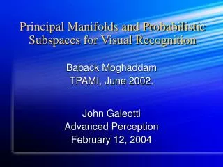
Principal Manifolds and Probabilistic Subspaces for Visual Recognition. Baback Moghaddam TPAMI, June 2002. John Galeotti Advanced Perception February 12, 2004. It’s all about subspaces. Traditional subspaces PCA ICA Kernel PCA (& neural network NLPCA) Probabilistic subspaces.

E N D
Principal Manifolds and Probabilistic Subspaces for Visual Recognition Baback Moghaddam TPAMI, June 2002. John Galeotti Advanced Perception February 12, 2004
It’s all about subspaces • Traditional subspaces • PCA • ICA • Kernel PCA (& neural network NLPCA) • Probabilistic subspaces
Linear PCA • We already know this • Main properties • Approximate reconstruction x ≈ y • Orthonormality of the basis T=I • Decorrelated principal components E{yiyj}i≠j = 0
Linear ICA • Like PCA, but the components’ distribution is designed to be sub/super Gaussian statistical independence • Main properties • Approximate reconstruction x ≈ Ay • Nonorthogonality of the basis A ATA≠I • Near factorization of the joint distribution P(y) P(y)≈ ∏ p(yi)
Nonlinear PCA (NLPCA) • AKA principal curves • Essentially nonlinear regression • Finds a curved subspace passing “through the middle of the data”
Nonlinear PCA (NLPCA) • Main properties • Approximate reconstruction y = f(x) • Nonlinear projection x ≈ g(y) • No prior knowledge regarding joint distribution of the components (typical) P(y) = ? • Two main methods • Neural network encoder • Kernel PCA (KPCA)
NLPCA neural network encoder • Trained to match the output to the input • Uses a “bottleneck” layer to force a lower-dimensional representation
KPCA • Similar to kernel-based nonlinear SVM • Maps data to a higher dimensional space in which linear PCA is applied • Nonlinear input mapping (x): NL, N<L • Covariance is computed with dot-products • For economy, make (x) implicit k(xi,xj) = ( (xi) (xj) )
KPCA • Does not require nonlinear optimization • Is not subject to overfitting • Requires no prior knowledge of network architecture or number of dimensions • Requires the (unprincipled) selection of an “optimal” kernel and its parameters
Nearest-neighbor recognition • Find labeled image most similar to N-dim input vector using a suitable M-dim subspace • Similarity ex: S(I1,I2) || ∆ ||-1, ∆ = I1 - I2 • Observation: Two types of image variation • Critical: Images of different objects • Incidental: Images of same object under different lighting, surroundings, etc. • Problem: Preceding subspace projections do not help distinguish variation type when calculating similarity
Probabilistic similarity • Similarity based on probability that ∆ is characteristic of incidental variations • ∆ = image-difference vector (N-dim) • ΩI = incidental (intrapersonal) variations • ΩE = critical (extrapersonal) variations
Probabilistic similarity • Likelihoods P(∆|Ω) estimated using subspace density estimation • Priors P(Ω) are set to reflect specific operating conditions (often uniform) • Two images are of the same object if P(ΩI|∆) > P(ΩE|∆) S(∆) > 0.5
Subspace density estimation • Necessary for each P(∆|Ω),Ω { ΩI, ΩE } • Perform PCA on training-sets of ∆ for each Ω • The covariance matrix (∑) will define a Gaussian • Two subspaces: • F = M-dimensional principal subspace of ∑ • F = non-principal subspace orthogonal to F • yi = ∆ projected onto principal eigenvectors • i = ranked eigenvalues • Non-principal eigenvalues are typically unknown and are estimated by fitting a function of the form f -n to the known eigenvalues
Subspace density estimation • 2(∆) = PCA residual (reconstruction error) • = density in non-principal subspace • ≈ average of (estimated) F eigenvalues • P(∆|Ω) is marginalized into each subspace • Marginal density is exact in F • Marginal density is approximate in F
Efficient similarity computation • After doing PCA, use a whitening transform to preprocess the labeled images into single coefficients for each of the principal subspaces: where and V are matrices of the principal eigenvalues and eigenvectors of either ∑I or ∑E • At run time, apply the same whitening transform to the input image
Efficient similarity computation • The whitening transform reduces the marginal Gaussian calculations in the principal subspaces F to simple Euclidean distances • The denominators are easy to precompute
Efficient similarity computation • Further speedup can be gained by using a maximum likelihood (ML) rule instead of a maximum a posteriori (MAP) rule: • Typically, ML is only a few percent less accurate than MAP, but ML is twice as fast • In general, ΩE seems less important than ΩI
Similarity Comparison Probabilistic Similarity Eigenface (PCA) Similarity
Experiments • 21x12 low-res faces, aligned and normalized • 5-fold cross validation • ~ 140 unique individuals per subset • No overlap of individuals between subsets to test generalization performance • 80% of the data only determines subspace(s) • 20% of the data is divided into labeled images and query images for nearest-neighbor testing • Subspace dimensions = d = 20 • Chosen so PCA ~ 80% accurate
Experiments • KPCA • Empirically tweaked Gaussian, polynomial, and sigmoidal kernels • Gaussian kernel performed the best, so it is used in the comparison • MAP • Even split of the 20 subspace dimensions • ME = MI = d/2 = 10 so that ME + MI = 20
Results Recognition accuracy (percent) N-Dimensional Nearest Neighbor (no subspace)
Results Recognition accuracy vs subspace dimensionality Note: data split 50/50 for training/testing rather than using CV
Conclusions • Bayesian matching outperforms all other tested methods and even achieves ≈ 90% accuracy with only 4 projections (2 for each class of variation) • Bayesian matching is an order of magnitude faster to train than KPCA • Bayesian superiority with higher resolution images verified in independent US Army FERIT tests • Wow! • You should use this
My results • 50% Accuracy • Why so bad? • I implemented all suggested approximations • Poor data--hand registered • Too little data Note: data split 50/50 for training/testing rather than using CV
My results • My data • His data