Download
1 / 32
320 likes | 407 Views
(H)MMs in gene prediction and similarity searches. What is an HMM? (Eddy2004). States Transition Probabilities Emission Probabilities. What is hidden? (Eddy2004). State Path. Log (product of transition and emission probabilities)

E N D
What is an HMM? (Eddy2004) • States • Transition Probabilities • Emission Probabilities
What is hidden? (Eddy2004) • State Path Log (product of transition and emission probabilities) Log (1 x 0.25 x 0.9 x 0.25 x 0.9 x 0.25 …0.9 x 0.4) = -41.22
What is hidden? (Eddy2004) • State Path
Using HMMs • Given the parameters of the model, compute the probability of a particular output sequence. This problem is solved by the forward algorithm. • Given the parameters of the model, find the most likely sequence of hidden states that could have generated a given output sequence. This problem is solved by the Viterbi algorithm. • Given an output sequence or a set of such sequences, find the most likely set of state transition and output probabilities. In other words, train the parameters of the HMM given a dataset of sequences. This problem is solved by the Baum-Welch algorithm.
Profile Hidden Markov Models • Statistical model of multiple sequence alignments • Position-specific description of the level of conservation and the probabilities of observing each type of amino acid (nucleotide) at that position • Protein domain alignments (PFAM, TIGRFams,…) • Regulator binding site alignments
Simple Profile HMM – no gaps Emission Probabilities determined from distribution of amino acids at each site of the alignment
Allowing gaps in a position-specific way Need to allow a sequence to contain one or more residues not found in the model (Insert) and also be missing regions that are present in the model (Delete)
Pfam • Database of protein domains and families available as multiple alignments and HMMs • Pfam-A is curated. Pfam-B is automated.
Pfam – scoring members • Trusted cut-off • Bit score for lowest scoring match included in the full alignment • Noise cut-off • Bit score for highest scoring match not included in the full alignment • Gathering cut-off
ATTTATCCGCCGAAGCCATTACATAGTATCGCGCTTGGCAGTCGGATTCCGGCGCTGCGTGAAGACTATA AACTTGGGCGTTTATGCGGTCGTTATTTCCTCGCCACGGTTGGCAAGCTATTAACTGAAAAAGCGCCGCT TACCCGCCATCTGGTGCCAGTGGTGACGCCGGAATCGATTGTCATTCCGCCTGCGCCAGTCGCCAACGAT ACGCTGGTTGCCGAAGTGAGCGACGCTCCGCAGGCGAACGACCCGACATTTAACAATGAGGATCTGGCTT GATTTGCCGTTTTATCGACACCCACTGCCATTTTGATTTCCCGCCGTTTAGTGGCGATGAAGAGGCCAGC CTGCAACGCGCGGCACAAGCGGGCGTAGGCAAGATCATTGTTCCGGCAACAGAGGCGGAAAATTTTGCCC GTGTGTTGGCATTAGCGGAAAATTATCAACCGCTGTATGCCGCATTGGGCTTGCATCCTGGTATGTTGGA AAAACATAGCGATGTGTCTCTTGAGCAGCTACAGCAGGCGCTGGAAAGGCGTCCGGCGAAGGTGGTGGCG GTGGGGGAGATCGGTCTGGATCTCTTTGGCGACGATCCGCAATTTGAGAGGCAGCAGTGGTTACTCGACG AACAACTGAAACTGGCGAAACGCTACGATCTGCCGGTGATCCTGCATTCACGGCGCACGCACGACAAACT GGCGATGCATCTTAAACGCCACGATTTACCGCGCACTGGCGTGGTTCACGGTTTTTCCGGCAGCCTGCAA CAGGCCGAACGGTTTGTACAGCTGGGCTACAAAATTGGCGTAGGCGGTACTATCACCTATCCACGCGCCA GTAAAACCCGCGATGTCATCGCAAAATTACCGCTGGCATCGTTATTGCTGGAAACCGACGCGCCGGATAT GCCGCTCAACGGTTTTCAGGGGCAGCCTAACCGCCCGGAGCAGGCTGCCCGTGTGTTCGCCGTGCTTTGC GAGTTGCGCCGGGAACCGGCGGATGAGATTGCGCAAGCGTTGCTTAATAACACGTATACGTTGTTTAACG TGCCGTAGGCCGGATAAGGCGTTCACGCCGCATCCGGCAGTTGGCGCACAATGCCTGATGCGACGCTTAA CGCGTCTTATCATGCCTACAGGTTTGTGCCGAACCGTAGGCCGGATAAGGCGTTCACGCCGCATCCGGCA GTTGGCGCACAATGCCTGATGCGACGCTTGTCGCGTCTTATCATGCCTACAAGTCTGTGCCGAACCGTAG GCCGGATAAGGCGTTCACGCCGCATCCGGCAGTCGGCGCATAATGCCTGATGCGACGCTTGTCGCGTCTTATCATGCCTACAGGTTTGTGCCGAACCGTAGGCCGGATAAGGCGTTCGCGCCGCATCCGGCAGTTGGCGC ACAATGCCTGATGCGACGCTTGACGCGTCTTATCAGGCCTACAAGTCTGTGCCGAACCGTAGGCCGTATC CGGCATGTCACAAATAGAGCGCCGGAAATATCAACCGGCTCACCCCGCGCACCTTTAACGCATCAGCCAACGGCTCAACGTCTTCCGGCGTGGCGCTCGCCCAGCTTTGCGCCTCGCCATACACGCCGTGGGCATGAAAC GCGTTCAGGCGTACCGGAACATCGCCGAGTCCCTTGATAAACGCCGCCAGTTCTTCGATGTGTTGCAAAT AATCCACCTGGCCAGGGATCACCAGCAAACGCAGTTCCGCCAGCTTGCCGCGCTCTGCCAGCAAATAGAT GCTGCGCTTAATCTGCTGATTATCGCGTCCGGTGAGTTGTTGATGACATTCGCTCCCCCACGCTTTGAGA TCGAGCATTGCGCCGTCGCACACCGGGAGCAATTTTTCCCAGCCGGTTTCGCTCAACATGCCGTTACTGT CCACCAGACAGGTGAGATGGCGCAGTTGCGGATCGTTTTTGATAGCAGTAAACAGCGCCACCACAAACGG CAGCTGGGTCGTGGCTTCACCGCCACTCACCGTTATCCCTTCGATAAACAGCACTGCTTTGCGGACATGG CTAAGCACTTCGTCCACGCTCATGGATTGCGCCATGGGCGTGGCATGTTGCGGACACCTCTTCAGGCAGG TATCACACTGCTCGCAAACCACAGCGTTCCACACCACTTTGCCGTCAACAATCTGCAACGCCTGATGCGG ACACTGTGGCACGCACTCCCCACAGTCATTGCAACGTCCCATCGTCCACGGATTGTGACAGTTTTTGCAG CGCAGATTGCAGCCCTGCAAAAACAGAGCCAGACGACTGCCTGGCCCGTCAACGCAGGAGAAGGGGATAA TCTTACTGACTAAAGCGCATCTGCTGTTCATGGCTTATCACGCGCGGCTGGCGTTCCAGAATACGAGTGT TGCGTGCGGCTTCTTCGCCCAGCCAGGTGGTGTTGGTGCGTGAACCTTCGGCGCGATATTTTTCTAAATC CGACAAACGCACCATATAACCGGTAACGCGAACCAGATCGTTACCGCTGACATTGGCGGTAAATTCACGC ATTCCGGCTTTAAAGGCACCGAGGCAAAGCTGTACCAGTGCCTGCGGGTTACGTTTGATGGTTTCGTCGA Gene Discovery
Prokaryotes: 10 kb DNA 3 mRNAs 9 proteins Eukaryotes: 10 kb DNA Unprocessed mRNA Processed mRNA 1 protein
Two Approaches • Ab initio • Based exclusively on computational models • Error prone, esp. for eukaryotes • Generally requires manual clean up • Comparative • Find genes corresponding to sequenced cDNAs • Find the genes already predicted for a closely related organism • If you can...use both strategies
Attributes that prove useful for gene prediction Begin with a start codon End with a stop codon Have a length divisible by 3 Splice sites Tend to have a species specific codon usage Exhibit even higher order biases in composition Tend to be more conserved between organisms than non-coding regions ORF Open Reading Frame
Detecting Signal Amid the Noise Each sequence can be translated in each of 6 reading frames, 3 for the sequenced strand and 3 for the reverse complement. There are far more open reading frames than there are genes. How do we know which reading frame contains real genes?
Codon usage in the E. coli K-12 and H. influenzae genomes 51.8%GC coding 38.1%GC coding Preference for GGC glycine codons Preference for GGU glycine codons
Gene Discovery using Markov Models and HMMs Example of a 1st order Markov model for gene prediction: The probability that base X is part of a coding region depends only on the base immediately preceding X. AX, TX, CX, GX How frequently does AX occur in a coding region vs. a non-coding region? A 5th order model: AAAAAX, AAAATX, AAAACX, … GGGGGX
Model Order – which is best? • In general, higher order models better describe the properties of real genes, but training higher order models requires more data and the training sets are limiting. • The probabilities of rare sequences in higher order models can be low enough that the model performs worse.
Gene Prediction Models based on Markov Chains • Basic Method: • Build at least 6 submodels (one for each reading frame) for coding regions and 1 for noncoding • Find ORFs -Start, Stop, mod(3) • Score each ORF by calculating the probability that it was generated by each model. Choose the model with the highest probability – if it exceeds a user-specified threshold, you have a gene. • Two popular applications: GLIMMER, GeneMark • Hidden Markov Models add modeling the gene boundaries as transitions between “hidden” states.
GLIMMER Reference:A.L. Delcher, D. Harmon, S. Kasif, O. White and S.L. Salzberg. Improved microbial gene identificaton with GLIMMERNAR, 1999, Vol. 27, No. 23, pp. 4636-4641. • GLIMMER can be “trained” using the genome itself • Finds the longest ORFs in the genome and assumes they are real genes to estimate emission probabilities • Interpolated Markov model • Not necessary to “fix” the order of the model • Analysis of 10 microbial genomes: • GLIMMER 2 finds 97.4-99.7% of annotated genes • PLUS another 7-25% !!! • GLIMMER 3 has a much lower False Positive Rate Specificity vs. Sensitivity
W.H. Majoros, M. Pertea, and S.L. Salzberg. TigrScan and GlimmerHMM: two open-source ab initio eukaryotic gene-finders http://www.tigr.org/software/GlimmerHMM/index.shtml Sensitivity: TP/(TP+FN) How much of what you hoped to detect did you get? Specificity: TP/(TP+FP) How much of what you detected is real?