Download
1 / 41
410 likes | 488 Views
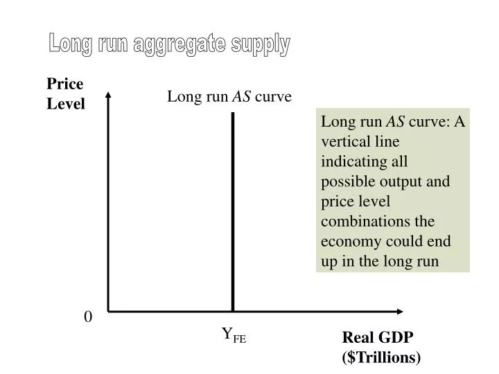
Long run aggregate supply. Price Level. Long run AS curve. Long run AS curve: A vertical line indicating all possible output and price level combinations the economy could end up in the long run. 0. Y FE. Real GDP ($Trillions). Self correcting mechanism. (How does it work?).

E N D
Long run aggregate supply PriceLevel Long run AS curve Long run AS curve: A vertical line indicating all possible output and price level combinations the economy could end up in the long run 0 YFE Real GDP($Trillions)
Self correcting mechanism (How does it work?) Some economists (Mankiw included) believe the economy is “self-correcting”—that is, forces are present that push the economy to long-run (or full-employment) equilibrium.
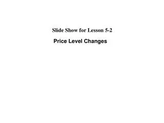
Long Run AS Curve AS2 PriceLevel AS1 Let AD shift from AD1 to AD2 P4 K P3 J P2 H P1 E AD2 AD1 0 YFE Y3 Y2 Real GDP($Trillions)
Change in short-run equilibrium Positive demand shock P and Y Y until Y =YFE Wage Rate Y > YFE Unit Cost P Long-run adjustment process
At point B, the price level is 140 and AS = $14 trillion. But equilibrium GDP is equal to $6 trillion when the price level is 140—we know this from the AD curve. • At point E, the price level is consistent with an output level of $10 along bothAS and AD curves Why is point E a short-run equilibrium? PriceLevel AS B 140 E 100 F AD 0 6 10 14 Real GDP($Trillions)
Fiscal Policy Fiscal policy is the use of the spending and taxing powers of government to influence total spending and thereby to stabilize real GDP, employment, and prices. The Employment Act of 1946 establishes a responsibility for the Federal government to “promote maximum employment, production, and purchasing power.
Effect of a Demand Shock Issue: Why did the economy move from point E to point H—instead of E to J? Increase in government spending PriceLevel AS 130 J H 100 E AD2 AD1 0 10 12 13.5 Real GDP($Trillions)
AD curve shifts rightward Multiplier Effect G GDP Movement along new AD curve Unit cost Money Demand Interest rate C and I P GDP Movement along AS curve Net result: GDP increases, but by less due to the effect of an increase in the price level
Effect of a decrease in taxes PriceLevel AS K 100 E S AD2 AD1 0 6.5 8 10 Real GDP($Trillions)
AD curve shifts rightward Multiplier Effect T↓ YD C GDP Movement along new AD curve Unit cost Money Demand Interest rate C and I P GDP Movement along AS curve Net result: GDP increases, but by less due to the effect of an increase in the price level
Monetary Policy The use of the instruments of monetary policy to change total spending in the economy and thereby influence total output and employment.
Effect of a decrease in the money supply PriceLevel AS K 100 E S AD2 AD1 0 6.5 8 10 Real GDP($Trillions)
AD curve shifts Leftward Interest rate C and I M GDP Movement along new AD curve Unit cost Money Demand Interest rate C and I P GDP Movement along AS curve Net result: GDP decreases, but by less due to the effect of an decrease in the price level
Conventional 30 year www.economagic.com
Monthly payments on a $110,000 30 year mortgage note 1 Does not include prorated insurance or property taxes.
Data in thousands of units www.economagic.gov
More recently, the Fed raised the federal funds rate six times between May 99 and May 2000—from 4.75% to 6.5 %.
The Fed reversed course at the beginning of 2001 and reduced the federal funds rate 11 times that year!
Supply shocks • The following factors could shift the (short-run) aggregate supply schedule up to the left: • An increase in the price of a basic commodity—e.g., petroleum, natural gas, wheat, soybeans. • An increase in average money wages and benefits not restricted to just one industry or sector of the economy. • An increase in the average markup over unit cost not restricted to just one industry or sector of the economy.
Effect of an increase in petroleum prices PriceLevel AS2 AS1 S 130 100 E AD2 AD1 0 6.5 8 10 Real GDP($Trillions)
I’d call that a shock, wouldn’t you? The storyof Joseph (see Old Testament)suggests buffer stocksas the remedy forsupply-shockinflation 1970s Oil Shock Price of One Barrel of 340 crude oil Source: The Petroleum Economist
Defining Productivity Productivity() means the average output of a workerper year, or alternatively: = GDP/Nwhere N is total employment and Y is real GDP. depends onthe efficiency withwhich labor is employedin the production ofgoods & services
Productivity and cost Let denote average annual compensation of employees (including benefits). Thus unit labor cost (UCL) is defined as: ULC = / Notice that compensationcan rise with no effect on ULC, so long as productivitykeeps pace
The Classical view of Fiscal policy Friends, we believe that fiscal policy is unnecessary and ineffective. The economy is doing just fine without meddling by Washington.
The Federal Budget The Federal budget is an annual statement of expenditures, tax receipts, and surplus or deficit of the government of the U.S. • Let: • G denote federal spending for goods and services in a fiscal year (Oct. 1 thru Sept. 30). • TX is federal tax receipts. • TR is federal transfer payments. • T is federal net taxes (TX - TR)
If G exceeds T in a fiscal year, then we have a federal deficit.If, however, T exceeds G, then we have a federal surplus.
Crowding Out • Crowding out is the idea that an increase in one component of spending will cause a decrease in other spending components. • An increase in G may cause a decrease in C, IP, or both—that is, government spending may “crowd out” private spending.
Crowding Out With an Initial Budget Deficit Total Supply of Funds (Saving) B • Increase in G = AH • Decrease in C = AC • Decrease in IP = CH 7% A C Interest Rate H 5% D2 = IP + G2 - T D1 = IP + G1 - T 0 1.75 2.05 2.25 Trillions of Dollars
Effects of a Reduction in the Government Surplus S2 = Savings + T – G2 S1 = Savings + T – G1 Interest Rate B 7% H C A 5% D = Investment 0 1.25 1.55 1.75 Trillions of Dollars
President Clinton’s economic strategy appears to have been effective in reducing interest rates