Download
1 / 48
480 likes | 571 Views
Geo-Routing Chapter 2. TexPoint fonts used in EMF. Read the TexPoint manual before you delete this box.: A A A A. Application of the Week: Mesh Networking ( Roofnet ). Sharing Internet access Cheaper for everybody S everal gateways fault-tolerance Possible data backup

E N D
Geo-RoutingChapter 2 TexPoint fonts used in EMF. Read the TexPoint manual before you delete this box.: AAAA
Application of the Week: Mesh Networking (Roofnet) • Sharing Internet access • Cheaper for everybody • Several gateways fault-tolerance • Possible data backup • Community add-ons • I borrow your hammer, you copy my homework • Get to know your neighbors
Rating • Area maturity • Practical importance • Theory appeal First steps Text book No apps Mission critical Boooooooring Exciting
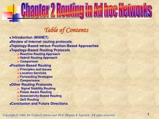
Overview • Classic routing overview • Geo-routing • Greedy geo-routing • Euclidean and Planar graphs • Face Routing • Greedy and Face Routing • 3D Geo-Routing
Classic Routing 1: Flooding • WhatisRouting? • „Routingistheact of movinginformationacross a networkfrom a source to a destination.“ (CISCO) • The simplest form of routing is “flooding”: a source s sends the message to all its neighbors; when a node other than destination t receives the message the first time it re-sends it to all its neighbors. + simple (sequence numbers) – a node might see the same message more than once. (How often?) – what if the network is huge but the target t sits just next to the source s? • We need a smarter routing algorithm s c b a t
Classic Routing 2: Link-State Routing Protocols • Link-state routing protocols are a preferred iBGP method (within an autonomous system) in the Internet • Idea: periodic notification of all nodes about the complete graph • Routers then forward a message along (for example) the shortest path in the graph + message follows shortest path – every node needs to store whole graph,even links that are not on any path – every node needs to send and receivemessages that describe the wholegraph regularly s c b a t
Classic Routing 3: Distance Vector Routing Protocols • The predominant method for wired networks • Idea: each node stores a routing table that has an entry to each destination (destination, distance, neighbor) • If a router notices a change in its neighborhood or receives an update message from a neighbor, it updates its routing table accordingly and sends an update to all its neighbors + message follows shortest path + only send updates when topology changes – most topology changesare irrelevant for a givensource/destination pair – every node needs to store a big table – count-to-infinity problem t? t=1 s c b a t t=2
Proactive Routing Protocols Both link-state and distance vector are “proactive,” that is, routes are established and updated even if they are never needed. If there is almost no mobility, proactive algorithms are superior because they never have to exchange information and find optimal routes easily. Reactive Routing Protocols Flooding is “reactive,” but does not scale If mobility is high and data transmission rare, reactive algorithms are superior; in the extreme case of almost no data and very much mobility the simple flooding protocol might be a good choice. Discussion of Classic Routing Protocols There is no “optimal” routing protocol; the choice of the routing protocol depends on the circumstances. Of particular importance is the mobility/data ratio.
Routing in Ad-Hoc Networks • Reliability • Nodes in an ad-hoc network are not 100% reliable • Algorithms need to find alternate routes when nodes are failing • Mobile Ad-Hoc Network (MANET) • It is often assumed that the nodes are mobile (“Car2Car”) • 10 Tricks 210 routing algorithms • In reality there are almost that many proposals! • Q: How good are these routing algorithms?!? Any hard results? • A: Almost none! Method-of-choice is simulation… • “If you simulate three times, you get three different results”
Geometric (geographic, directional, position-based) routing • …even with all the tricks there will be flooding every now and then. • In this chapter we will assume that the nodes are location aware (they have GPS, Galileo, or an ad-hoc way to figure out their coordinates), and that we know where the destination is. • Then we simply route towards the destination t s
Geometric routing • Problem: What if there is no path in the right direction? • We need a guaranteed way to reach a destination even in the case when there is no directional path… • Hack: as in floodingnodes keep trackof the messagesthey have alreadyseen, and then theybacktrack* from there *backtracking? Does this mean that we need a stack?!? t ? s
Alice Bob Geo-Routing: Strictly Local ???
Greedy Geo-Routing? Alice Bob
Greedy Geo-Routing? Bob ? Carol
What is Geographic Routing? • A.k.a. geometric, location-based, position-based, etc. • Each node knows its own position and position of neighbors • Source knows the position of the destination • No routing tables stored in nodes! • Geographic routing makes sense • Own position: GPS/Galileo, local positioning algorithms • Destination: Geocasting, location services, source routing++ • Learn about ad-hoc routing in general
Greedy routing • Greedy routinglooks promising. • Maybe there is away to choose thenext neighborand a particulargraph where we always reach thedestination?
Examples why greedy algorithms fail • We greedily route to the neighborwhich is closest to the destination:But both neighbors of x arenot closer to destination D • Also the best angle approachmight fail, even in a triangulation:if, in the example on the right,you always follow the edge withthe narrowest angle to destinationt, you will forward on a loopv0, w0, v1, w1, …, v3, w3, v0, …
Euclidean and Planar Graphs • Euclidean: Points in the plane, with coordinates, e.g. UDG • UDG: Classic computational geometry model, special case of disk graphs • All nodes are points in the plane, two nodes are connected iff (if and only if) their distance is at most 1, that is {u,v} 2 E , |u,v| · 1 + Very simple, allows for strong analysis – Not realistic: “If you gave me $100 for each paper written with the unit disk assumption, I still could not buy a radio that is unit disk!” – Particularly bad in obstructed environments (walls, hills, etc.) • Natural extension: 3D UDG
Euclidean and Planar Graphs • Planar: can be drawn without “edge crossings” in a plane • A planar graph already drawn in the plane without edge intersections is called a plane graph. In the next chapter we will see how to make a Euclidean graph planar.
Breakthrough idea: route on faces • Remember thefaces… • Idea: Route along the boundaries of the faces that lie on the source–destination line
Face Routing 0. Let f be the face incident to the source s, intersected by (s,t) • Explore the boundary of f; remember the point p where the boundary intersects with (s,t) which is nearest to t; after traversing the whole boundary, go back to p, switch the face, and repeat 1 until you hit destination t.
“Right Hand Rule” Face Routing Properties • All necessary information is stored in the message • Source and destination positions • Point of transition to next face • Completely local: • Knowledge about direct neighbors‘ positions sufficient • Faces are implicit • Planarity of graph is computed locally (not an assumption) • Computation for instance with Gabriel Graph
Face routing is correct • Theorem: Face routing terminates on any simple planar graph in O(n) steps, where n is the number of nodes in the network • Proof: A simple planar graph has at most 3n–6 edges. You leave each face at the point that is closest to the destination, that is, you never visit a face twice, because you can order the faces that intersect the source—destination line on the exit point. Each edge is in at most 2 faces. Therefore each edge is visited at most 4 times. The algorithm terminates in O(n) steps. Definition: f 2O(g) → 9 c>0, 8 x>x0: f(x) ≤ c·g(x)
Face Routing • Theorem: Face Routing reaches destination in O(n) steps • But: Can be very bad compared to the optimal route
Is there something better than Face Routing? How can we improve Face Routing?
Is there something better than Face Routing? • How to improve face routing? A proposal called “Face Routing 2” • Idea: Don’t search a whole face for the best exit point, but take the first (better) exit point you find. Then you don’t have to traverse huge faces that point away from the destination. • Efficiency: Seems to be practically more efficient than face routing. But the theoretical worst case is worse – O(n2). • Problem: if source and destination are very close, we don’t want to route through all nodes of the network. Instead we want a routing algorithm where the cost is a function of the cost of the best route in the unit disk graph (and independent of the number of nodes).
Adaptive Face Routing (AFR) • Idea: Useface routingtogether with“growing radius”trick: • That is, don’troute beyondsome radius r by branchingthe planar graphwithin an ellipseof exponentiallygrowing size.
AFR Example Continued • We grow theellipse andfind a path
AFR Pseudo-Code 0. Calculate G = GG(V) Å UDG(V)Set c to be twice the Euclidean source—destination distance. • Nodes w 2 W are nodes where the path s-w-t is larger than c. Do face routing on the graph G, but without visiting nodes in W. (This is like pruning the graph G with an ellipse.) You either reach the destination, or you are stuck at a face (that is, you do not find a better exit point.) • If step 1 did not succeed, double c and go back to step 1. • Note: All the steps can be done completely locally,and the nodes need no local storage.
The (1) Model • We simplify the model by assuming that nodes are sufficiently far apart; that is, there is a constant d0 such that all pairs of nodes have at least distance d0. We call this the (1) model. • This simplification is natural because nodes with transmission range 1 (the unit disk graph) will usually not “sit right on top of each other”. • Lemma: In the (1) model, all natural cost models (such as the Euclidean distance, the energy metric, the link distance, or hybrids of these) are equal up to a constant factor. • Remark: The properties we use from the (1) model can also be established with a backbone graph construction.
Analysis of AFR in the (1) model • Lemma 1: In an ellipse of size c there are at most O(c2) nodes. • Lemma 2: In an ellipse of size c, face routing terminates in O(c2) steps, either by finding the destination, or by not finding a new face. • Lemma 3: Let the optimal source—destination route in the UDG have cost c*. Then this route c* must be in any ellipse of size c* or larger. • Theorem: AFR terminates with cost O(c*2). • Proof: Summing up all the costs until we have the right ellipse size is bounded by the size of the cost of the right ellipse size.
Lower Bound • The network on the rightconstructs a lower bound. • The destination is thecenter of the circle, the source any nodeon the ring. • Finding the right chaincosts (c*2), even for randomizedalgorithms • Theorem: AFR is asymptotically optimal.
Non-geometric routing algorithms • In the (1) model, a standard flooding algorithm enhanced with growing search area idea will (for the same reasons) also cost O(c*2). • However, such a flooding algorithm needs O(1) extra storage at each node (a node needs to know whether it has already forwarded a message). • Therefore, there is a trade-off between O(1) storage at each node or that nodes are location aware, and also location aware about the destination. This is intriguing.
GOAFR – Greedy Other Adaptive Face Routing • Back to geometric routing… • AFR Algorithm is not very efficient (especially in dense graphs) • Combine Greedy and (Other Adaptive) Face Routing • Route greedily as long as possible • Circumvent “dead ends” by use of face routing • Then route greedily again Other AFR: In each face proceed to pointclosest to destination
GOAFR+ – Greedy Other Adaptive Face Routing • Early fallback to greedy routing: • Use counters p and q. Let u be the node where the exploration of the current face F started • p counts the nodes closer to t than u • q counts the nodes not closer to t than u • Fall back to greedy routing as soon as p > ¢ q (constant > 0) • Theorem: GOAFR is still asymptotically worst-case optimal… • …and it is efficient in practice, in the average-case. • What does “practice” mean? • Usually nodes placed uniformly at random
Average Case • Not interesting when graph not dense enough • Not interesting when graph is too dense • Critical density range (“percolation”) • Shortest path is significantly longer than Euclidean distance too sparse critical density too dense
Critical Density: Shortest Path vs. Euclidean Distance • Shortest path is significantly longer than Euclidean distance • Critical density range mandatory for the simulation of any routing algorithm (not only geographic)
Randomly Generated Graphs: Critical Density Range 1.9 1 0.9 1.8 Connectivity 0.8 1.7 0.7 1.6 0.6 Greedy success 1.5 Shortest Path Span Frequency 0.5 1.4 0.4 Shortest Path Span 1.3 0.3 1.2 0.2 1.1 0.1 critical 1 0 10 15 0 5 Network Density [nodes per unit disk]
Simulation on Randomly Generated Graphs 1 10 AFR worse 0.9 9 0.8 8 Connectivity 0.7 7 0.6 Greedy success 6 Frequency 0.5 Performance 5 0.4 GOAFR+ 4 0.3 3 0.2 better 2 0.1 critical 0 1 0 2 4 6 8 10 12 Network Density [nodes per unit disk]
A Word on Performance • What does a performance of 3.3 in the critical density range mean? • If an optimal path (found by Dijkstra) has cost c, then GOAFR+ finds the destination in 3.3¢c steps. • It does not mean that the path found is 3.3 times as long as the optimal path! The path found can be much smaller… • Remarks about cost metrics • In this lecture “cost” c = c hops • There are other results, for instance on distance/energy/hybrid metrics • In particular: With energy metric there is no competitive geometric routing algorithm
s t GOAFR: Summary Face Routing Adaptive Face Routing Greedy Routing GOAFR+ Average-case efficiency Worst-case optimality “Practice” “Theory”
3D Geo-Routing • The world is not flat. We can certainly envision networks in 3D, e.g. in a large office building. Can we geo-route in three dimensions? Are the same techniques possible? • Certainly, if the node density is high enough (and the node distribution is kind to us), we can simply use greedy routing. But what about those local minima?!? • Is there something like a face in 3D? • The picture on the right is the 3Dequivalent of the 2D lowerbound, proving that we need at least OPT3 steps.
3D Geo Routing It is proven that no deterministic k-local routing algorithm for 3D UDGs exist. Deterministic: Whenever a node n receives a message from node m, n determines the next hop as a function f(n,m,s,t,N(n)), where s and t are the source and the target nodes and N(n) the neighborhood of n. k-local: A node only knows its k-hop neighborhood How would you do 3D routing?
Routing with and without position information • Without position information: • Flooding does not scale • Distance Vector Routingdoes not scale • Source Routing • increased per-packet overhead • no theoretical results, only simulation • With position information: • Greedy Routing may fail: message may get stuck in a “dead end” • Geometric Routing It is assumed that each node knows its position
Summary of Results • If position information is available geo-routing is a feasible option. • Face routing guarantees to deliver the message. • By restricting the search area the efficiency is OPT2. • Because of a lower bound this is asymptotically optimal. • Combining greedy and face gives efficient algorithm. • 3D geo-routing is impossible. • Even if there is no position information, some ideas might be helpful. • Geo-routing is probably the only class of routing that is well understood. • There are many adjacent areas: topology control, location services, routing in general, etc.
Open problem • Geo-routing is one of the best understood topics. In that sense it is hard to come up with a decent open problem. Let’s try something wishy-washy. • We have seen that for a 2D UDG the efficiency of geo-routing can be quadratic to an optimal algorithm (with routing tables). However, the worst-case example is quite special. • Open problem: How much information does one need to store in the network to guarantee only constant overhead? • Variant: Instead of UDG some more realistic model • How can one maintain this information if the network is dynamic?