Download
1 / 56
610 likes | 979 Views
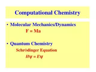
Computational Quantum Chemistry Part I. Obtaining Properties. Properties are usually the objective. May require accurate, precisely known numbers Necessary for accurate design, costing, safety analysis Cost and time for calculation may be secondary

E N D
Properties are usually the objective. • May require accurate, precisely known numbers • Necessary for accurate design, costing, safety analysis • Cost and time for calculation may be secondary • Often, accurate trends and estimates are at least as valuable • Can be correlated with data to get high-accuracy predictions • Can identify relationships between structure and properties • A quick, sufficiently accurate number or trend may be of enormous value in early stages of product and process development, for for operations, or for troubleshooting • Great data are best; but also theory-based predictions
Phase and reaction equilibria Bond and interaction energies Ideal-gas thermochemistry Thermochemistry and equations of state for real gases, liquids, solids, mixtures Adsorption and solvation Reaction kinetics Rate constants, products Transport properties Interaction energies, dipole µ, kthermal, DAB Analytical information Spectroscopy: Frequencies, UV / Vis /IR absorptivity GC elution times Mass spectrometric ionization potentials and cross-sections, fragmentation patterns NMR shifts Mechanical properties of hard and soft condensed matter Electronic and optical properties of solids What properties do we want?
Restate: What kind of properties come directly from computational quantum chemistry? • Energies, structures optimized with respect to energy, harmonic frequencies, and other properties based on zero-kelvin electronic structures • Interpret with theory to get derived properties and properties at higher temperatures • The theoretical basis for most of this translation is Quantum-mechanical energies Statistical mechanics
Simplest properties are interaction energies: Here, the van der Waals well for an Ar dimer.
Simplest chemical bonds are much stronger. UB3LYP/6-311++G(3df,3dp) with basis-set superposition error correction
At zero K, define the dissociation energy D0 as the well depth less zero-point energy. Alternate view is that D0 = E0(dissociated partners) - [E0(molecule) + ZPE], where ZPE is the zero-K energy of the stretching vibration.
Geometry is then found by optimizing computed energy with respect to coordinates (here, 1).
Vibrational frequencies (at 0 K) are calculated using parabolic approximation to well bottom. • How many? Need 3Natoms coordinates to define molecule • If free translational motion in 3 dimensions, then three translational degrees of freedom • Likewise for free rotation: 3 d.f. if nonlinear, 2 if linear • Thus, 3Natoms-5 (nonlinear) or 3Natoms-6 (nonlinear) vibrations • For diatomic, ∂2E/∂r2 = force constant k [for r dimensionless] • F (= ma = m∂2r/∂t2) = -kr is a harmonic oscillator in Newtonian mechanics (Hooke’s law) • Harmonic frequency is (k/m)1/2/2π s-1 or (k/m)1/2/2πc cm-1 (wavenumbers) • For polyatomic, analyze Hessian matrix [∂2E/∂ri∂rj] instead
Next, determine ideal-gas thermochemistry. • Start with ∆fH0° and understand how energies are given • We recognize that energies are not absolute, but rather must be defined relative to some reference • We use the elements in their equilibrium states at standard pressure, typically 1 atm or 1 bar (0.1 MPa): • From ab initio calculations, energy is typically referenced to the constituent atoms, fully dissociated. Get ∆fH0° from:
To go further, we need statistical mechanics. • The partition function q(V,T)=∑exp(-i /T) arises naturally in the development of Maxwell-Boltzmann and Bose-Einstein statistics • Quantum mechanics gives the quantized values of energy and thus the partition functions for: • Translational degrees of freedom • External rotational degrees of freedom (linear or nonlinear rotors) • Rovibrational degrees of freedom (stretches, bends, other harmonic oscillators, and internal rotors) • Electronic d.f. require only electronic and degeneracy.
Entropy, energy, and heat capacity can be expressed in terms of the partition function(s).
Simplest treatment is of ideal gas, beginning with the translation degrees of freedom. • Quantum mechanics for pure translation in 3-D gives: • Note the standard-state pressure in the last equation
Rigid-rotor model for external rotation introduces the moment of inertia I and rotational symmetry ext.
Add harmonic oscillators with frequencies i and electronic degeneracy of go. • For each harmonic oscillator, • It is convenient to redefine zero for vibrational energy as zero rather than 0.5h; this shift requires the zero-point energy correction to energy. As a result, • If only the ground electronic state contributes, then (Cvo)elec=0 and (So)elec=R·ln go. Otherwise, need g1 & 1.
Taken together, they give us ideal-gas Cpo and So, and integration over T gives ∆fH298o. • Even for gases, there are further complications beyond the Rigid-Rotor Harmonic Oscillator model (RRHO) • Low-frequency modes may be fully excited • Anharmonic behaviors like free and hindered internal rotors • We can generally deal with the statistical mechanics that complicate these issues • Computational chemistry even can calculate anharmonicities like shape of the potential well or barriers to rotation • Likewise, we can calculate terms needed to model thermochemistry of liquids, solutions, and solids • Likewise for phase equilibrium and transport properties.
Now examine kinetics from quantum chemistry. • We have already discussed how to locate transition states along the “minimum energy path”: • A stationary point (∂E/∂ = 0) with respect to all displacements • A minimum with respect to all displacements except the one corresponding to the reaction coordinate • More precisely, all but one eigenvalue of the Hessian matrix of second derivatives are positive (real frequencies) or zero (for the overall translational and rotational degrees of freedom • The exception: Motion along the reaction coordinate • It corresponds to a frequency ‡ that is an imaginary number • If eitis a sinusoidal oscillation, then ‡ is exponential change
The entire minimum energy path may not be a simple motion, but the transition state is still separable. Potential energy surface for O-O bond fission in CH2CHOO· B3LYP/6-31G(d); Kinetics analysis based on O-O reaction-coordinate-driving calculation at B3LYP/6-311+G(d,p)
Consider transition-state thermochemistry. • It has a geometrical structure, electronic state, and vibrations, so assume we can calculate q‡, H‡, S‡, Cp‡ • For classical transition-state theory, Eyring assumed: • At equilibrium, TS would obey equilibrium relations with reactant • The reaction coordinate would be a separable degree of freedom • Thus, with it treated as a 1-D translation or a vibration, • Recognizing the form of a thermochemical Keq,
Computational quantum chemistry gives very useful numbers for Eact, also can give good A-factor. • For gas kinetics, calculate H‡, S‡, Cp‡, ∆S‡(T), ∆H‡(T) • Reaction coordinate contributes zero to S‡ • Standard-state correction is necessary for bimolecular reactions • Eact, like bond energy, may be adequate for comparisons • Most other factors can be handled • If reaction coordinate involves H motion and low T, quantum-mechanical tunneling may occur (use calculated barrier shape) • High-pressure limit is required (use RRKM, Master Equation) • Low-frequency modes like internal rotors give the most uncertainty in ∆S‡, but we can calculate barriers • In principle, the same for anharmonicity of vibrations
Other properties are predicted, too; Advances in methods have been aided by demand. • Good semi-empirical and ab initio calculations for excited states give pigment and dye behaviors • Solvation models by Tomasi and others make liquid-phase behaviors more calculable • Hybrid methods have proven powerful • QM/MM for biomolecule structure and ab-initio molecular dynamics for ordered condensed phases; calculate interactions as dynamics calculations proceed • Spatial extrapolation such as embedded-atom models of catalysts and Morokuma’s ONIOM method; connect or extrapolate domains of different-level calculations
Computational Quantum ChemistryPart II. Principles and Methods. In parallel, see the faces behind the names.
“Ab initio” is widely but loosely used to mean “from first principles.” • Actually, there is considerable use of assumed forms of functionalities and fitted parameters. • John Pople noted that this interpretation of the Latin is by adoption rather than intent. In its first use: • The two groups of Parr, Craig, and Ross [J Chem Phys 18, 1561 (1951)] had carried out some of the first calculations separately across the Atlantic - and thus described each set of calcs as being ab initio!
Three key features of theory are required for ab initio calculations. • Understand how initial specification of nuclear positions is used to calculate energy • Solving the Schrödinger equation • Understand “basis sets” and how to choose them • Functions that represent the atomic orbitals • e.g., 3-21G, 6-311++G(3df,2pd), cc-pVTZ • Understand levels of theory and how to choose them • Wavefunction methods: Hartree-Fock, MP4, CI, CAS • Density functional methods: LYP, B3LYP, etc. • Compound methods: CBS, G3 • Semiempirical methods: AM1, PM3
Initially, restrict our discussion to an isolated molecule. • Equivalent to an ideal gas, but may be a cluster of atoms, strongly bonded or weakly interacting. • Easiest to think of a small, covalently bonded molecule like H2 or CH4in vacuo. • Most simply, the goal of electronic structure calculations is energy. • However, usually we want energy of an optimized structure and the energy’s variation with structure.
Begin with the Hamiltonian function, an effective, classical way to calculate energy. • Express energy of a single classical particle or an N-particle collection as a Hamiltonian function of the 3N momenta pj and 3N coordinates qj (j=1,N) such that: where: H = Kinetic Energy (T) + Potential Energy (V) = Total Energy
For quantum mechanics, a Hamiltonian operator is used instead. • Obtain a Hamiltonian function for a wave using the Hamiltonian operator: to obtain: where Y is the “wavefunction,” an eigenfunction of the equation • Born recognized that Y2 is the probability density function
For quantum molecular dynamics, retain t; Otherwise, t-independent. • Separation of variables gives Y(q) and thus the usual form of the Schroedinger or Schrödinger equation: • If the electron motions can be separated from the nuclear motions (the Born-Oppenheimer approximation), then the electronic structure can be solved for any set of nuclear positions.
Easiest to consider H atom first as a prototype. e- • Three energies: • Kinetic energy of the nucleus. • Kinetic energy of the electron. • Proton-electron attraction. • With more atoms, also: • Internuclear repulsion • Electron-electron repulsion. • Electrons are in specific quantum states called orbitals. • They can be in excited states (higher-energy orbitals). proton
Restate the nonrelativistic electronic Hamiltonian in atomic units. • With distances in bohr (1 bohr = 0.529 Å) and with energies in hartrees (1 hartree = 627.5 kcal/mol), where (After Hehre et al., 1986) • [Breaks down when electrons approach the speed of light, the case for innermost electrons around heavy atoms]
Set up Y, the system wavefunction. • Need functionality (form) and parameters. • (1) Use one-electron orbital functions (“basis functions”) to ... • (2) Compose the many-electron molecular orbitals y by linear combination, then ... • (3) Compose the system Y from y’s. • Wavefunction Y must be “antisymmetric” • Exchanging identical electrons in Y should give -Y • Characteristic of a “fermion”; vs. “bosons” (symmetric)
H-atom eigenfunctions y correspond to hydrogenic atomic orbitals.
Construct each MO yi by LCAO. • Lennard-Jones (1929) proposed treating molecular orbitals as linear combinations of atomic orbitals (LCAO): • Linear combination of s orbital on one atom with s or p orbital on another gives s bond: • Linear combination of p orbital on one atom with p orbital on another gives p bond:
Molecular Y includes each electron. • First, include spin (x=-1/2,+1/2) of each e-. • Define a one-electron spin orbital, c(x,y,z,x) composed of a molecular orbital y(x,y,z) multiplied by a spin wavefunction a(x) or b(x). • Next, compose Y as a determinant of c’s. <- Electron 1 in all c’s; <- Electron 2 in all c’s; <- Electron n in all c’s • Interchange row => Change sign; \ Functionally antisymmetric.
However, basis functions fi need not be purely hydrogenic - indeed, they cannot be. • Form of basis functions must yield accurate descriptions of orbitals. • Hydrogenic orbitals are reasonable starting points, but real orbitals: • Don’t have fixed sizes, • Are distorted by polarization, and • Involve both valence electrons (the outermost, “bonding” shell) and non-valence electrons. • Hydrogenic s-orbital has a cusp at zero, which turns out to cause problems.
Simulate the real functionality (1). • Start with a function that describes hydrogenic orbitals well. • Slater functions; e.g., • Gaussian functions; e.g., • No s cusp at r=0 • However, all analytical integrals • Linear combinations of gaussians; e.g., STO-3G • 3 Gaussian “primitives” to simulate a STO • (“Minimal basis set”)
Simulate the real functionality (2). • Allow size variation. • Alternatively, size adjustment only for outermost electrons (“split-valence” set) to speed calcs • For example, the 6-31G set: • Inner orbitals of fixed size based on 6 primitives each • Valence orbitals with 3 primitives for contracted limit, 1 primitive for diffuse limit • Additional very diffuse limits may be added (e.g., 6-31+G or 6-311++G)
Simulate the real functionality (3). • Allow shape distortion (polarization). • Usually achieved by mixing orbital types: • For example, consider the 6-31G(d,p) or 6-31G** set: • Add d polarization to p valence orbitals, p character to s • Can get complicated; e.g., 6-311++G(3df,2pd)
Simulate the real functionality (4). • A noteworthy improvement is the set of Complete Basis Set methods of Petersson. • Better parameterization of finite basis sets. • Extrapolation method to estimate how result changes due to adding infinitely more s,p,d,f orbitals • Another basis-set improvement is development of Effective Core Potentials. • As noted before, for transition metals, innermost electrons are at relativistic velocities • Capture their energetics with effective core potentials • For example, LANL2DZ (Los Alamos N.L. #2 Double Zeta).
The third aspect is solution method. • Hartree-Fock theory is the base level of wavefunction-based ab initio calculation. • First crucial aspect of the theory: The variational principle. • If Y is the true wavefunction, then for any model antisymmetric wavefunction F, E(F)>E(Y). Therefore the problem becomes a minimization of energy with respect to the adjustable parameters, the Cµi’s and l’s.
The Hartree-Fock result omits electron-electron interaction (“electron correlation”). • The variational principle led to the Roothaan-Hall equations (1951) for closed-shell wavefunctions: or • ei is diagonal matrix of one-electron energies of the yi. • F, the Fock matrix, includes the Hamiltonian for a single electron interacting with nuclei and a self-consistent field of other electrons; S is an atomic-orbital overlap matrix. • All electrons paired (RHF); there are analogous UHF equations.
One improvement is to use “Configuration Interaction”. • Hartree-Fock theory is limited by its neglect of electron-electron correlation. • Electrons interact with a SCF, not individual e’s. • “Full CI” includes the Hartree-Fock ground-state determinant and all possible variations. • The wavefunction becomes where s includes all combinations of substituting electrons into H-F virtual orbitals. • The a’s are optimized; not so practical.
Partial CI calculations are feasible. • CIS (CI with Singles substitutions), CISD, CISD(T) (CI with Singles, Doubles, and approximate Triples) • CI calculations where the occupied ci elements in the SCF determinant are substituted into virtual orbitals one and two at a time and excited-state energies are calculated. • CASSCF (Complete Active Space SCF) is better: Only a few excited-state orbitals are considered, but they are re-optimized rather than the SCF orbitals. • Other variants: QCISD, Coupled Cluster methods.
Perturbation Theory is an alternative. • Møller and Plesset (1934) developed an electronic Hamiltonian based on an exactly solvable form H0 and a perturbation operator: • A consequence is that the wavefunction Y and the energy are perturbations of the Hartree-Fock results, including electron-electron correlation effects that H-F omits. • Most significant: MP2 and MP4.
Compound methods aim at extrapolation. • The G1, G2, and G3 methods of Pople and co-workers calculate energies in cells of their matrix, then project more accurately. • G2 gave ave. error in ∆Hf of ±1.59 kcal/mol. • G3 gives ave. error in ∆Hf of ±1.02 kcal/mol. • CBS methods are compound methods that give impressive results. • Melius and Binkley’s BAC-MP4 is based on MP4/6-31G(d,p)//HF/6-31G(d) calculation.
Besides energy, calculations give electron density, HOMO, LUMO. • Electron density (from electron probability density function = Y2) is an effective representation of molecular shape. • Each molecular orbital is calculated, including highest-energy occupied MO (HOMO) and lowest-energy unoccupied MO (LUMO) • HOMO-LUMO gap is useful for Frontier MO theory and for band gap analysis.
Results can be seen with ethylene. Calculations and graphics at HF/3-21G* with MacSpartan Plus (Wavefunction Inc.). Electron density HOMO; LUMO