Download
1 / 26
260 likes | 325 Views
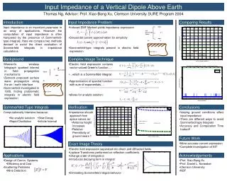
Modeling a Dipole Above Earth. Saikat Bhadra Advisor : Dr. Xiao-Bang Xu Clemson SURE 2005. Overview. Objective Problem Background & Theory Results Problems in the EIT Model Concluding Remarks. Objective. Accurate modeling of a dipole Linear Antenna Lossy Earth Material Properties

E N D
Modeling a Dipole Above Earth Saikat Bhadra Advisor : Dr. Xiao-Bang Xu Clemson SURE 2005
Overview • Objective • Problem Background & Theory • Results • Problems in the EIT Model • Concluding Remarks
Objective • Accurate modeling of a dipole • Linear Antenna • Lossy Earth • Material Properties • Scientific Model • K. Sarabandi, M. D. Casciato, and I. KohEfficient Calculation of the Fields of A Dipole Radiating Above an Impedance Surface
Solving Electromagnetic Problems • The Emag Bible : Maxwell’s Equations • Available in integral and differential forms • Vector Potential • Links Magnetic and Electric Fields
Non-flat & non-Euclidean surfaces Time Varying Layered Materials Antenna Environment Inhomogeneous Materials Location : Austin, TX
Simplifications • Simplify math and assume : • Flat Earth Model • Two Layers • Upper half space – “air” • Lower half space – lossy earth • Euclidean (rectangular) geometry • Infinitesimal Vertical Dipole • Superposition to extend to finite dipoles
Observation Point Dipole Free Space Impedance Half Space Electric Field • In this type of problem, two fields are involved • Direct Electric Fields • Fields due to antenna radiating • Solution in closed form & well documented • Diffracted Electric Fields • Fields from antenna that are reflecting off the lower surfaces • Subject of research since 1909
Original Solution – Diffracted Fields • Arnold Sommerfeld (1909) • Sommerfeld Integrals • Non-analytic • Numerical integration difficult • Requires asymptotic techniques • Valid for certain regions • Convergence difficult
Exact Image Theory Solution • Sarabandi, Casciato, Koh (2002) • Source Equation :
EIT Formulation • Separate diffracted and direct components • Reflection Coefficients transformed using Laplace transform • Bessel function identities
Observation Point Direct Dipole Free Space Diffracted Impedance Half Space EIT Solution – Diffracted Fields
EIT Solution • Integral Advantages • Rapidly Decays • Non-Oscillatory • Easy numerical evaluation after exchange of integration and differentiation
Dipole Dipole Dipole Dipole Dipole Dipole Exact Image Theory Observation Point Direct Free Space Diffracted Impedance Surface
Finite Length Dipoles • Sarabandi’s model uses infinitesimal dipole • Finite dipole can be approximated by a sum of infinitesimal dipoles • Superposition Principle
Calculating Input Impedance • Induced EMF Method : • Current distribution assumed to sinusoidal • Transmission line approximation • Inaccurate when dipole comes close to half space
Numerical Techniques • Gaussian Integration • Useful in many emag problems • Handles singular integrands better • More accurate than rectangular, trapezoidal, and Simpson’s rule • Integral Truncation • Can’t numerically evaluate an infinite integral • Vectorized Code
Results • Computational time varies with antenna location • Frequency independence • Asymptotically approaches original antenna impedance
Problems of the EIT Model • Recall the breakdown of electric field into diffracted and direct components • Diffracted fields should go to zero if the half-space is removed • There is no longer any surface for waves to bounce off of • Numerical Results disagree • Currently finding theoretical errors of the model
Concluding Remarks • EIT model could be promising but problems need to be solved • Research Applications • Antenna Design • Integral Equations & Numerical Methods
Future Work • Solve the EIT model problems • Extend the problem to dipoles of arbitrary orientation • Develop more accurate model of current distribution • Investigate different source models
Acknowledgments • Dr. Xu • Dr. Noneaker
Environmental Variables • Time varying • Inhomogeneous Materials (x,y) • Water • Grass • Concrete • Layered Materials (z) • Trees, Grass, Soil • Non-flat surfaces • Amorphous (non-Euclidean) geometries • Mutual Coupling