Download
1 / 59
590 likes | 773 Views
The CMB and Gravity Waves. John Ruhl Case Western Reserve University. 3/17/2006, CERCA at St. Thomas. WMAP 3yr temperature maps… what the sky really looks like. 23 GHz. 61 GHz. 33 GHz. 94 GHz. 41 GHz. (What the sky really looks like). WMAP 3-year map, “galaxy subtracted”.

E N D
The CMB and Gravity Waves John Ruhl Case Western Reserve University 3/17/2006, CERCA at St. Thomas
WMAP 3yr temperature maps… what the sky really looks like. 23 GHz 61 GHz 33 GHz 94 GHz 41 GHz (What the sky really looks like)
Boomerang “T” maps B03: 150GHz (published) 10’ resolution, ~1000 sq. deg.
Acbar maps 150GHz, 5’ resolution, 10’s of sq. deg, More coming soon.
<TT> Power spectra=> CDM looks good Power Spectrum (uK2) Legendre l
WMAP(3yr)+others <TT> Figure 18, Hinshaw etal, WMAP 3-year release
WMAP 3yr data… theory-scaled to high-ell… Fig 5, Spergel etal, WMAP 3-year release
“Post B03”(pre-WMAP3)parameters MacTavish etal, B03 release
Still of interest r = T/S: primordial gravity waves (tensor modes) nT: spectral index of tensor mode power spectrum ns: spectral index of density perturbation power spectrum, Dark Energy w, w’, etc non-gaussianity Isocurvature modes Suprises: eg “not flat”, obs. disagreements, etc.
CMB“goal” ns vs r : current limits WMAP 3yr, r<0.28 (95%CL) w/SDSS r T/S ns Plot from M. Tegmark, TFCR report
CMB polarization Two causes: “Normal” CDM: Density perturbations at z=1000 lead to velocities that create local quadrupoles seen by scattering electrons. => “E-mode polarization” (no curl) Gravity waves: create local quadrupoles seen by scattering electrons, => “B-mode polarization” (curl)
Both are caused by the polarization dependence in Thomson scattering
Anisotropic illumination => polarization Green = probability of emitting in that direction… Observer Vertical pol. Line of sight No emission to observer Line of sight Horizontal pol.(in and out of page) Line of sight
Gravity waves at z=1000 Gravity Wave Surface of last scattering
Flavors of CMB polarization Two patterns: Density perturbations: curl-free, “E-mode” Gravity waves: curl, “B-mode”
Linear polarization Stokes parameters IAU convention for Q and U North North - East - East + + U Q Each point on the sphere has a Q or U value determined by the polarization at that point.
Stokes Parameters vs. E and B mode The E-mode (or B-mode) value at a point on the sphere depends on the polarization pattern all around it. Direction you’re looking on the sky (2 components) Same thing, but variable for integration Polar coordinates of relative to Weighting function (Note: w=0 for theta =0)
For a given circle ( ), circumference goes as , while , so the contribution of that circle goes as 1/ . E and B mode patterns Blue = + Red = - “local” Q “local” U
E and B mode patterns E-mode Unchanged under parity flip B-mode Sign reverses under parity flip Seljak and Zaldarriaga, astro-ph/9805010
E-mode polarization (simulation) Seljak and Zaldarriaga, astro-ph/9805010 Color: |E| Bars: E-mode polarization direction and size
B-mode polarization (simulation) Seljak and Zaldarriaga, astro-ph/9805010 Color: |B| Bars: B-mode polarization direction and size
Reionization bump Primordial B-modes CMB Polarization power spectra Shape and amplitude of EE are predicted by CDM. ``Shape” of BB is predicted “scale-invariand GW’s”. Amplitude of BB is model dependent.
Fig 22, Hinshaw etal, WMAP 3yr release WMAP <TE>, Kogut etal
EE power spectrum data Figure 22, Page etal, WMAP 3-yr release.
WMAP Polarization data Current “high-l” BB limits BB limit (1sigma) Foreground model r=0.3 BB Figure 25, Page etal, WMAP 3yr release
The Future of CMB polarization measurements Foregrounds Technology
Synchrotron Dust Foregrounds at l=50 r = 0.01 S. Golwala, 2005
Galactic Foregrounds: l-space From G. Hinshaw, TFCR report
“Future, large angular scale” CMB Polarization Experimentsdeployedfunded proposed Quad: NTD bolo, 90/150 GHz, ~0.2deg, ~100 elements. Spole. Bicep: NTD bolo, 90/150 GHz, ~1deg, ~100 elements, Spole Ebex: SC Bolos, 90-400GHz, ~0.2deg, ~1000 elements, balloon Pappa: SC bolos, 90/150GHz, ~1deg, ~20 elements, balloon Clover: SC bolos?, 90-220GHz?, ~1deg, ~1000 elements, Chile Quiet: Hemts, ??? freqs/elements, Chile Polarbear: SC bolos, 90/150/220GHz, ~0.2deg, ~? Elements, Chile Spider: SC bolos, 40-220GHz, ~1deg, ~1000 elements, balloon CMBPOL: ???, satellite [see TFCR (aka “Weiss”) report]
Sensitivities 1 10 100 1000 1 10 100 1000 Plot from T. Montroy
Predicted Future Experiment Sensitivities From G. Hinshaw, TFCR report
Systematics to conquer Table 6.1 from TFCR report
On-chip modulator(continuous) modulator photons Detector feed(s) Other optics “on chip”
“After primary” modulator(continuous) feed(s) Other optics photons Detector modulator “on chip”
“Ideal” Future experiment to probe Inflation • Lots of sensitive detectors and integration time • “Good enough” angular resolution (to measure l=100 bump) • “Large enough” sky coverage (to measure reionization bump) • Low systematics, polarization modulator… optimized for Polarization. Ultimate instrument: CMBPOL satellite Realistic (proposed) instrument…
Spider(CMBPOL on a rope) Canada: U. Toronto, U.BC UK: Cardiff, Imperial Coll. London USA: Caltech, Case, JPL, NIST A balloone-borne“low l” machine
Six frequency bandsSix telescopesClean refractor opticsHalfwave plates
CIT/JPL Polarized Array8x8=64 pixel phased-array “patches”, 2 polarizations on each.
Around the world flight from Australia, night time observing only Large sky coverage => get to low l
Spider baseline bands and sensitivities 6 bands 1856 detectors