Download
1 / 26
260 likes | 494 Views
Quantifying Patterns of Biological Diversity using Vertebrate Habitat Models. Frank A. La Sorte. Acknowledgements. Southwest Regional Gap Analysis Project: Bruce C. Thompson, Kenneth G. Boykin, Scott Schrader, Robert A. Deitner.

E N D
Quantifying Patterns of Biological Diversity using Vertebrate Habitat Models Frank A. La Sorte
Acknowledgements Southwest Regional Gap Analysis Project: Bruce C. Thompson, Kenneth G. Boykin, Scott Schrader, Robert A. Deitner. New Mexico Cooperative Fish and Wildlife Research Unit, New Mexico State University.
Justification • We require tools to quantify large scale patterns of biological diversity • provide information for decision making on large scale environmental issues • Adequately documenting these patterns is inherently difficult • tremendous ecological complexity • lack of time and resources
Justification (continued) • Trade off: • document large scale patterns quickly with limited precision, accuracy, generality, and predictability • Gap analysis presents regional patterns of vertebrate habitat associations within their estimated ranges • However, it lacks well defined methods for: • quantifying diversity • decision making
Objectives • Concept of Ecological Diversity • Dimensions and Components • Quantifying Diversity Patterns within Gap Analysis • Richness, Evenness, Distinctness • Example: 1996 New Mexico Gap Data • New Mexico • Tularosa Basin • Applications for Decision Making
Limitations • Models are subjective, non-probabilistic, and static • Accuracy unknown • Level of error propagation unknown • Variables highly correlated • Qualitative (presence/absence) • Limited to vertebrates • Varying perceptions of scale by species • Habitat is scale dependent • No intra- and interspecific factors • Ignores size and spatial arrangement of patches
Ecological Diversity • Units • Grain • Extent • Diversity patterns • Richness • Evenness • Taxonomic distinctness • Landscape patterns • Time
Distinctness Order Family Evenness Genus Richness Species Diversity Patterns
Vertebrate Habitat Models • Large scale biological and abiotic features, that can be represented cartographically, found within the estimated range of a species • Combined with Boolean AND operators to create a binary grid (presence/absence)
Gap Richness • Definition: quantity of vertebrate habitats within a unit area • Sum all vertebrate habitat models
Richness • Does not predict presence, persistence, fitness, habitat quality, or biodiversity • Interpretation of richness “hotspots” problematic • Not consistent across taxa • Scale dependent • Biased towards marginal populations
Gap Evenness • Definition: How evenly vertebrate habitat is distributed within a taxonomic level in a unit area • Species as the unit of evenness • Summarize evenness trend with principle component analysis
Evenness Metrics • Non-ordered or scalar metrics • Ordered metrics • Information theory (Rényi, Hill) • Cumulative measures (Lorenz curve)
Lorenz Curve Lorenz Curve: (0, 0) (1/s, p1) (2/s, p1 + p2)…(s-1/s, p1 + p2 + … + ps-1) (1, 1) Where the proportions are ranked p1< p2<…< ps for s groups Gini Coefficient: (Area between the Lorenz Curve and the line of equality) x 2
Order Family ω = 1 ω = 2 ΣΣ i<jωij s (s – 1)/2 ω = 3 Δ+ = Genus Species Gap Taxonomic Distinctness • Definition: How taxonomically distinct vertebrate habitat is within a unit area • Measured as the average taxonomic path length for each cell based upon a weighting factor (Clarke & Warwick 1998) Path length weights (ω) Average path length
Example: New Mexico • NM GAP 1996 • 100 x 100 m cells • 346 vertebrate species • 20 Orders • 55 Families • 195 Genera
Example: Tularosa Basin Alamogordo White Sands National Monument Sacramento Mountains 9,369.2 km2
High Low Richness Taxonomic distinctness Evenness Order Family
Application to decision making • Provides more detailed information on the patterns of diversity • multivariate nature of diversity • Use a combination of diversity components with other variables to: • more accurately represent gaps • contrast sites based upon some criteria • locate sites with desired characteristics
Decision Making • Assist in directing policy, research, management, and conservation efforts more efficiently • Should not be the sole source of information • Should be interpreted cautiously and honestly