Download

1 / 47
520 likes | 863 Views
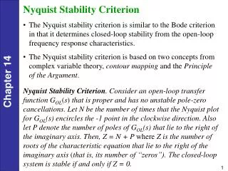
Nyquist Stability Criterion. By: Nafees Ahmed Asstt . Prof., EE Deptt , DIT, Dehradun. Introduction . Nyquist criterion is used to identify the presence of roots of a characteristic equation of a control system in a specified region of s-plane.

E N D
Nyquist Stability Criterion By: Nafees Ahmed Asstt. Prof., EE Deptt, DIT, Dehradun By: Nafees Ahmed, EED, DIT, DDun
Introduction • Nyquist criterion is used to identify the presence of roots of a characteristic equation of a control system in a specified region of s-plane. • A closed loop system will be stable if pole of closed loop transfer function (roots of characteristic equation) are on LHS of s-plane • From the stability view point the specified region being the entire right hand side of complex s-plane. Note: An open loop unstable system may become stable if it is a closed loop system By: Nafees Ahmed, EED, DIT, DDun
Introduction… • Although the purpose of using Nyquist criterion is similar to Routh-Hurwitz criterion but the approach differ in following respects: • The open loop transfer function G(s)H(s) is considered instead of closed loop characteristic equation • Inspection of graphical plot of G(s)H(s) enables to get more than Yes or No answer of Routh-Hurwitz method pertaining to stability of control systems. • Nyquist stability criterion is based on the principle of argument. The principle of argument is related with the theory of mapping . By: Nafees Ahmed, EED, DIT, DDun
Mapping • Mapping from s-plane to G(s)H(s) plane 1.Consider a single valued function G(s)H(s) of s • s is being traversed along a line though points sa=1+j1 & sb=2.8+j0.5 By: Nafees Ahmed, EED, DIT, DDun
Mapping… By: Nafees Ahmed, EED, DIT, DDun
Mapping… • Note: • For s-plane • The zero of the transfer function is at s=-1.5 in s-plane • A Phasor Ma is drawn from the point s=-1.5 to the point sa. • The magnitude Ma & Phase φa of this phasor gives the value of the G(s)H(s) at sa in polar form. • Similarly the magnitude Mb & Phase φb of the phasor gives the value of the G(s)H(s) at sb in polar form • For G(s)H(s)-plane • The magnitude & phasor of the transfer function G(s)H(s)=s+1.5 at a point in G(s)H(s) plane is given by the magnitude and the phase of the phasor drawn from the origin of G(s)H(s)-plane. By: Nafees Ahmed, EED, DIT, DDun
Mapping… 2.Consider another single valued function G(s)H(s) of s • Here s is varied along a closed path (sa→sb→sc→sd→sa) in clockwise direction as shown in figure. • Zero z1 is inside while z2 is outside the specified path By: Nafees Ahmed, EED, DIT, DDun
Mapping… By: Nafees Ahmed, EED, DIT, DDun
Mapping… • Note: from s-plane • φ1 is the phase angle of phasor M1 (=sa-z1) at sa • φ2 is the phase angle of phasor M2 (=sa-z2) at sa • The phasor M1 undergoes a change of -2π i.e. one clockwise rotation • The phase M2 undergoes a changes of zero i.e. No rotation By: Nafees Ahmed, EED, DIT, DDun
Mapping… • Note: from G(s)H(s) plane • While traversing sa→sb→sc→sd→sa, corresponding change in Phasor will be along the path Ma→Mb→Mc→Md→Ma, i.e. one complete rotation w.r.torigin • So the phasor change in function[G(s)H(s)=(s+z1)(s+z2)] is also -2π i.e. one clockwise rotation in G(s)H(s) plane. By: Nafees Ahmed, EED, DIT, DDun
Mapping… • Therefore, if the number of zeros of G(s)H(s) in a specified region in s-plane is Z and the independent variable s is varied along a path closing the boundary of such a region in clockwise direction the corresponding change in the argument (Phase) of G(s)H(s) in G(s)H(s)-plane is -2πZ (clockwise) • On similar reasoning, if the number of poles of G(s)H(s) in a specified region in s-plane is P and the independent variable s is varied along a path closing the boundary of such a region in clockwise direction the corresponding change in the argument (Phase) of G(s)H(s) in G(s)H(s)-plane is +2πP (anti clockwise) By: Nafees Ahmed, EED, DIT, DDun
Mapping… • Consider Z zeros & P Poles of G(s)H(s) together as located inside a specified region in s-plane and s being varied as mentioned above, the mathematical expression for corresponding change in the argument of G(s)H(s) in G(s)H(s) plane is • It is know as principle of argument By: Nafees Ahmed, EED, DIT, DDun
Determination of Zeros of G(s)H(s) which are located inside a specified region in s-plane By: Nafees Ahmed, EED, DIT, DDun
Determination of Zeros of G(s)H(s) which are located inside a specified region in s-plane… By: Nafees Ahmed, EED, DIT, DDun
Determination of Zeros of G(s)H(s) which are located inside a specified region in s-plane… By: Nafees Ahmed, EED, DIT, DDun
Determination of Zeros of G(s)H(s) which are located inside a specified region in s-plane… By: Nafees Ahmed, EED, DIT, DDun
Application of Nyquist Criterion to determine the stability of closed loop system • The overall T.F of a closed loop sys • G(s)H(s) is open loop T.F. • 1+ G(s)H(s)=0 is the characteristic equation • Let By: Nafees Ahmed, EED, DIT, DDun
Application of Nyquist Criterion to determine the stability of closed loop system… • So G(s)H(s) & 1+ G(s)H(s)=0 are having same poles but different zeros • Zeros of 1+ G(s)H(s)=0 =>roots of it • For stable system roots(zeros) of characteristic equation should not be on RHS of s-plane. • Thus the basis of applying Nyquist criterion for ascertaining stability of a control system is that, the specified region for identifying the presence of zeros of 1+ G(s)H(s)=0 should be the entire RHS of s-plane By: Nafees Ahmed, EED, DIT, DDun
Application of Nyquist Criterion to determine the stability of closed loop system… • The path along which s is varied is shown bellow (called Nyquist Contour) By: Nafees Ahmed, EED, DIT, DDun
Application of Nyquist Criterion to determine the stability of closed loop system… • For the above path, mapping is done in G(s)H(s) and change in argument of G(s)H(s) plane is noted • So no of zeros of G(s)H(s) on RHS of s-plane is calculated by • Note: • Above procedure calculates the no of roots of G(s)H(s) not the 1+G(s)H(s)=0 • However the no of roots of 1+ G(s)H(s)=0 can be find out if the origin (0,0) of G(s)H(s) pane is shifted to the point (-1,0) in G(s)H(s) plane. • Origin is avoided from the path By: Nafees Ahmed, EED, DIT, DDun
Application of Nyquist Criterion to determine the stability of closed loop system… • So no of zeros and poles of 1+G(s)H(s)=0 on RHS of s-plane is related with the following expression • Where • N=No of encirclement of (-1+j0) by G(s)H(s) plot. (The -ve direction of encirclement is clockwise) • P+=No of poles of G(s)H(s) with + real part • Z+=No of zeros of G(s)H(s) with + real part • For stable control system Z+=0 And generally P+=0 => N=0 => No encirclement of point -1+j0 By: Nafees Ahmed, EED, DIT, DDun
Closing Nyquist plot from s=-j0 to s=+j0 • Consider the following example • Draw it polar plot • Put ω=+0 • Assuming1>>j0T • Put ω=+∞ • Assuming1<<j ∞ T • Separate the real & imj parts • So No intersection with jω axis other then at origin and infinity By: Nafees Ahmed, EED, DIT, DDun
Closing Nyquist plot from s=-j0 to s=+j0… • Polar plot ⇒ω=+0 to ω=+∞ • Plot for variation from ω=-0 to ω=-∞ is mirror image of the plot from ω=+0 to ω=+∞. As shown by doted line. • From ω=-0 to ω=+0 the plot is not complete. The completion of plot depends on the no of poles of G(s)H(s) at origin(Type of the G(s)H(s)). By: Nafees Ahmed, EED, DIT, DDun
Closing Nyquist plot from s=-j0 to s=+j0… • For closing ω=-0 to ω=+0 • Consider a general transfer function • As s→0 By: Nafees Ahmed, EED, DIT, DDun
Closing Nyquist plot from s=-j0 to s=+j0… • s is varied in s-plane from s=-0 to s=+0 in anti clockwise direction as shown above such that r→0. By: Nafees Ahmed, EED, DIT, DDun
Closing Nyquist plot from s=-j0 to s=+j0… • The equation of phasor along the semi-circular arc will be • Put the value of s in equ (2) • In s-plane • At s=-j0 ϴ=-π/2 • At s=+j0 ϴ=+π/2 • So change in ϴ =(+π/2)-(-π/2)=+π By: Nafees Ahmed, EED, DIT, DDun
Closing Nyquist plot from s=-j0 to s=+j0… • The corresponding change in phase of G(s)H(s) in G(s)H(s) plane is determined below: • At s=-j0, ϴ=-π/2; put in equation (3) • At s=+j0, ϴ=+π/2; put in equation (3) • So corresponding change By: Nafees Ahmed, EED, DIT, DDun
Closing Nyquist plot from s=-j0 to s=+j0… • Hence, if in the s-plane s changes from s=-j0 to s=+j0 by π radian (anti-clockwise) then the corresponding change in phase of G(s)H(s) in G(s)H(s) plane is –nπ (clockwise) and the magnitude of G(s)H(s) during this phase change is infinite. • Where • n=Type of the system i.e. no of poles at origin By: Nafees Ahmed, EED, DIT, DDun
Closing Nyquist plot from s=-j0 to s=+j0… • The closing angle for different type of sys By: Nafees Ahmed, EED, DIT, DDun
Examples: • Example 1: Examine the closed loop stability using Nyquist Stability criterion of a closed loop system whose open loop transfer function is given by • Sol: As discussed previously it Polar (Nyquist) plot will be as shown By: Nafees Ahmed, EED, DIT, DDun
Example1… • System is type 1=> plot is closed from ω=-0 to ω=+0 through an angle of –π (clockwise) with an infinite radius By: Nafees Ahmed, EED, DIT, DDun
Example1… • no of roots of characteristic equation having + real part(Z+) are given by • N=0 As point -1+j0 is not encircled by the plot • P+=0 (Poles G(s)H(s) having + real parts) • Hence closed loop system is stable By: Nafees Ahmed, EED, DIT, DDun
Example 2:The open loop transfer function of a unity feedback control is given below • Determine the closed loop stability by applying Nyquist criterion. • Sol: Draw it Polar plot, put s=jω, H(jω)=1 By: Nafees Ahmed, EED, DIT, DDun
Example 2… • Put ω=+0 • Put ω=+∞ • Separate the real & imj parts • intersection with real axis, put Imj=0 • Real part By: Nafees Ahmed, EED, DIT, DDun
Example 2… • As the system is type 2 the Nyquist plot from ω=-0 to ω=+0 is closed through an angle of 2π in clockwise direction By: Nafees Ahmed, EED, DIT, DDun
Example 2… • N=-2 (as point (-1+j0) is encircled twice clockwise) • P+=0(No poles with +real part) • So By N=P+-Z+=> -2=0-Z+ =>Z+=2 • No of roots having + real parts are 2 • => Closed loop unstable system By: Nafees Ahmed, EED, DIT, DDun
Example 3 • Determine the stability by Nyquist stability criterion of the system • Sol: • As it is type 1 system so • Nyquist plot from ω=-0 • to ω=+0 is closed • through an angle of • π in clockwise direction By: Nafees Ahmed, EED, DIT, DDun
Example 3… • N=-1, P+=1 • N=P+-Z+ =>Z+=2 (Two roots on RHS of s-plane) • So closed loop system will be unstable By: Nafees Ahmed, EED, DIT, DDun
Gain Margin, Phase Margin, Gain crossover freq, Phase crossover freq By: Nafees Ahmed, EED, DIT, DDun
Gain Margin, Phase Margin, Gain crossover freq, Phase crossover freq… • Phase Crossover Frequency (ωp) : The frequency where a polar plot intersects the –ve real axis is called phase crossover frequency • Gain Crossover Frequency (ωg) : The frequency where a polar plot intersects the unit circle is called gain crossover frequency So at ωg By: Nafees Ahmed, EED, DIT, DDun
Gain Margin, Phase Margin, Gain crossover freq, Phase crossover freq… • Phase Margin (PM): • Phase margin is that amount of additional phase lag at the gain crossover frequency required to bring the system to the verge of instability (marginally stabile) Φm=1800+Φ Where Φ=∠G(jωg) if Φm>0 => +PM (Stable System) if Φm<0 => -PM (Unstable System) By: Nafees Ahmed, EED, DIT, DDun
Gain Margin, Phase Margin, Gain crossover freq, Phase crossover freq… • Gain Margin (GM): • The gain margin is the reciprocal of magnitude at the frequency at which the phase angle is -1800. In terms of dB By: Nafees Ahmed, EED, DIT, DDun
Stability • Stable: If critical point (-1+j0) is within the plot as shown, Both GM & PM are +ve GM=20log10(1 /x) dB By: Nafees Ahmed, EED, DIT, DDun
Stability … • Unstable: If critical point (-1+j0) is outside the plot as shown, Both GM & PM are -ve GM=20log10(1 /x) dB By: Nafees Ahmed, EED, DIT, DDun
Stability … • Marginally Stable System: If critical point (-1+j0) is on the plot as shown, Both GM & PM are ZERO GM=20log10(1 /1)=0 dB By: Nafees Ahmed, EED, DIT, DDun
Relative stability • GMsystem1=GMsystem2 • But • PMsystem1>PMsystem2 • So • system 1 • is more stable By: Nafees Ahmed, EED, DIT, DDun
Books • Linear Control System By B.S. Manke • Khanna Publication By: Nafees Ahmed, EED, DIT, DDun