Download

1 / 51
510 likes | 624 Views
How long do we need to run an experiment?. Ignacio Colonna & Don Bullock. Grain yield maps show a considerable variability across years. Yield map. Algorithm NF = 21.4 kg N / MT grain * YG – Rotation Credit – Incidental N. Yield response function.

E N D
How long do we need to run an experiment? Ignacio Colonna & Don Bullock
Grain yield maps show a considerable variability across years Yield map Algorithm NF = 21.4 kg N / MT grain * YG – Rotation Credit – Incidental N
Yield response function • But is the variability in yield that matters? • It is the variability in response to inputs that matters. • Assuming a profit-maximizing farmer…
Yield response and profit functions (only due to N)
Different curves, same optimum Similar curves, different optima • Statistics vs. management: • Responses may be significantly different statistically, yet yield similar management decisions.
But these are ‘after the fact’ optimum N rates… • Farmers’ decisions usually based on the best a priori guess • Concept of ex-post vs ex-ante optima • Ex-post optimum: computed after collecting the data • Ex-ante optimum: best guess given the information available before the fact. (“long-run” optimum) • e.g. we have 15 years of N response data for a site:
For this study • Question 1: • How does the uncertainty about the ‘true’ N rate at a given site change with years of experimentation? • No published estimates on uncertainty in ex-ante N rates as a function of experiment length in the US Midwest.
Question 2: What is the cost of not knowing the true N rate at a given site? No published estimates on practical consequences of different lengths of experimentation on fertilizer application decisions.
Data : source • N fertilizer trial at Monmouth, IL • (conducted by Nafziger,Adee,Hoeft,Mainz)
Data : experimental design • 21 years : 1983-2003 • Split plot in RCBD, 3 reps. • 2 rotations: C/C and C/S • 5 fertilizer rates: 0, 67, 134, 201, 269 kg/ha (pre-plant) • Individual plots 6.1 m 18 m
21 years x 2 Rotations: Raw Yield Means ( C/S C/C
21 years x 2 Rotations: Model fits C/S C/C Yield response (ton/ha)
21 years x 2 Rotations: Variability in ex-post N opt ‘True’ ex-ante Nopt=173 kg/ha ‘True’ ex-ante Nopt=110 kg/ha
A look at uncertainty in ex-ante N optima Pick two years at random (#1) Compute ex-ante optimum N rate (#1) Pick two years at random (#2) Compute ex-ante optimum N rate (#2). Pick two years at random (#3) 1000 samples=1000 estimates of ex-ante N rate Repeat for groups of 3 years,4 years,…etc.
Results from resampling approach: distributions Ex-ante optimum N (kg/ha)
Results from resampling approach: SD and CV C/C Ex-ante Nopt std.deviation Ex-ante Nopt CV C/S Years of experimentation Years of experimentation
Results fromresamplingapproach: Practical implications C/C Error (+ or -)
Results from resampling approach: Practical implications C/C Loss relative to maximum Profit at ‘true’ ex- ante Nopt= 249 $/ha
Conclusions so far : • Relatively small effect in monetary terms (~very small for >4 years, e.g. at 4 years < 10% prob of loss > 10$/ha • But, how do these errors compare with within-field spatial variability in Nopt? • Is this of use to conventional systems?
Regression of Crop Yield with Soil and Landscape Attributes: An Assessment of Some Common Methods for Dealing with Spatially Correlated Residuals
Spatial correlation of residuals in regressions are often overlooked in agronomic and engineering research, especially so in analyses related to precision agriculture, with a few exceptions. We argue that this oversight is not trivial and neither is the choice for its solution.
Soybean yield monitor data (2 years) 1999 2001
Soil sample data (P and K)
Elevation data and derivatives (Slope, Aspect, etc.)
Spatial Mixed GLS: Generalized Least Squares estimator • Errors not assumed independent. • Σestimated with geostatistical models. • Parameters for Sest by ML or REML Example of code in SAS® Proc Mixed *Iterative. Initial values obtained from inspection of variogram of OLS residuals parms/*sill*/(600)/*range*/(90)/ *nugget*/(650); repeated /subject=intercept local type=sp(sph)(x y); OLS(Ordinary least squares) if errors are as assumed, but often residuals do show spatial correlation due to variables not included in the model
Spatial Mixed GLS: Generalized Least Squares estimator Errors not assumed independent. Σestimated with geostatistical models. Parameters for Sest by ML or REML
Nearest Neighbors (non-iterative version – computations are simple) Average of neighboring OLS residuals Computation: • Compute OLS regression Y=Xb+e and save residuals (e). • Compute average of neighboring residuals for each point (We). • Compute new OLS regression but using We from 2 as a covariate in: Y=Xb+ gWe +x.
Spatially autoregressive approaches SAR error - the effect of the observed OLS residuals is due to the omission of spatially structured explanatory variables in the X matrix. SAR lag -value of response variable is in part due to a contagion or diffusion from the same variable at nearby locations or there is a mismatch between the scale at the a variable is measured and the true scale of the process. Decide upon model based on substantive interpretation and Lagrange Multiplier specification tests (Anselin).
Red: Point i Yellow: neighbors = 1 Blue: not neighbors = 0 “Queen Structure” for W
SAR-Error(Spatial Autoregressive – Error) Average of neighboring OLS residuals
SAR-Lag(Spatial Autoregressive – Lag) Average of neighboring values for Y “Direct effect of neighbors on point i”
Points shifted vertically to aid visualization. Flat line→spatially uncorrelated residuals. All methods seem to achieve similar results in terms of residual spatial structure.
Shaded values are significantly different from OLS estimates Shaded values are significantly different from OLS estimates
Regression example - Conclusions Spatial Mixed, SAR-error and SAR-lag parameter estimates showed significant differences to those from OLSonly for the year with the largest spatial structure. Parameter estimates from NN where not significantly different from OLS ones, despite the apparent difference in magnitude.
Estimates from SAR-lag were in general smaller in magnitude relative to all other methods. This is due to the “filtering” performed by this method on the response variable. Is this reasonable for this type of analysis? We believe it is not.
So, which method should we choose to account for the spatial correlation of residuals in regression? This question motivates the second partof our analysis.
3 independent variables: x1,x2 and e with • short and long range error structures:
Random values for each variable generated at 4 densities in a 400 m x 400 m field. • Values generated using Sim2d in SAS®. Based on LU decomposition of the covariance matrix. • Spatial structure based on a spherical model. • 1000 realizations for each variable-density-error structure combination (e.g. e-440-short range)
= + + • Generate dependent variable Y: • Yshort=10+0.6 x1+1.2 x2+eshort • Ylong=10+0.6 x1+1.2 x2+eshort • Adjusted theoretical R2=0.37 1000 X y e x1 x2
Methodology: Analysis of simulated data • Regression model: Y=b0+b1 x1+b2 x2 • Parameters Estimated by • OLS • Spatial Mixed • SAR-error • SAR-lag • Nearest neighbors
Higher point densities: • Dispersion: OLS and NN show a considerably higher dispersion than Spatial Mixed and SAR methods. • Bias: SAR-lag shows a marked downward bias at high densities, resulting in an underestimation of the true effect of x1. • Lower point densities: • Neither dispersion nor bias differ among methods for a short correlation range. • For a larger correlation range in the residuals, dispersion for OLS and bias for SAR-lag are still important at lower densities. • Results are similar for b2 (not shown) SAR-lag bias SAR-lag bias
Spatial structure effect SAR-lag bias SAR-lag bias
Conclusions from simulationsn (partial) The inadequate use of a SAR-lag model can generate a considerable downward bias in parameter estimates. The meaningfulness of such model for regression analysis of agronomic data as in the example above may be questionable (i.e. there is no direct “influence of neighbors yield on yield at point i”).
Spatial Mixed and SAR-error resulted in similar outcomes when the latter was based on a “Queen” neighbors matrix. The use of other matrices proved inefficient (not shown), while the results for Spatial Mixed were consistent even when the covariance model used was incorrect (e.g. exponential instead of spherical).