Download

1 / 23
230 likes | 351 Views
Lecture 6: Windowing of DFT. Instructor: Dr. Gleb V. Tcheslavski Contact: gleb@ee.lamar.edu Office Hours: Room 2030 Class web site: http://ee.lamar.edu/gleb/dsp/index.htm. by Steve Higgins. The idea of windowing. - not really practical. (6.2.1).

E N D
Lecture 6: Windowing of DFT Instructor: Dr. Gleb V. Tcheslavski Contact:gleb@ee.lamar.edu Office Hours: Room 2030 Class web site: http://ee.lamar.edu/gleb/dsp/index.htm by Steve Higgins
The idea of windowing - not really practical (6.2.1) What if we observe an infinitely long sequence over a finite length time window? Than we don’t see the rest of the signal. 0 D-1 Let D is the number of samples (data points) observed.
Windowing; what it causes - a windowed view of xn (6.3.1) where: (6.3.2) ynis a D- sequence (finite length), therefore, we can evaluate its DFT. (6.3.3) periodic convolution property Therefore,is a “dispersed/convoluted/obscured view of zero-padded length (6.3.4)
Windowing; what it causes (cont) (6.4.1) (6.4.2) If 0[-, ] (6.4.3) delay due to a center of the window (6.4.4)
Leakage (6.5.1) (6.5.2) Let D = 100 Spectrum of a rectangular window This is what causes so called “leakage” – observation of frequency components that do not exist in the spectrum of the signal – Due to observation only!
Frequency sampling DFT means “frequency sampling”! We can only observe specific frequency components of the sinc curve, and, therefore, can see only the specific frequency components of our signal! Zero-padding increases number of observed frequency samples. BUT! our sinusoid leaves at 0 and this is the only frequency where we expect it to be! Therefore, by “smart” choice of P we can observe the signal ONLY at 0 and at the zero-crossings, i.e. at (6.5.1)
Characteristics of window functions Windows characteristics Peak Side Lobe level (PSL), dB Side Lobe Roll-off (SLR), dB/octave Main lobe width (MLW) at xx dB
Characteristics of window functions Windows characteristics We want: • MLW – narrow for better spectral resolution • PSL – lower to have less masking for nearby components • SLR – “better” (faster) to have less masking for far away components
Multiple sinusoids (6.9.1) (6.9.2) Assume for simplicity that m = 0 for every m. (6.9.3) (6.9.4) As a consequence, for two equal amplitude sinusoids, we will observe 2 peaks of |Yk| “about” half the time (depending on relative phase) when the frequency difference is: - Rayleigh limit of frequency resolution – related to the window! (6.9.5)
Multiple sinusoids Two sinusoids at the Rayleigh limit… Phase shift 0o Phase shift 90o
Multiple sinusoids Phase shift 180o Two sisoids are NOT resolved! They appear as a single peak in the frequency domain!
Multiple sinusoids DFTs of two sinusoids of different frequencies and different magnitudes. DFT of their sum…
Multiple sinusoids Masking – one signal is obscured by another in the freq. domain We need a “better” window!
Multiple sinusoids Alternative – von Hann window Two sins can be resolved!!
Multiple sinusoids Two windows comparison
Different DFT windows Rectangular (Boxcar) window (6.14.1)
Different DFT windows von Hann (Hanning) window (6.15.1)
Different DFT windows Hamming window (6.16.1)
Different DFT windows Blackman window (6.17.1)
Different DFT windows Kaiser window (6.18.1)
Different DFT windows Different windows comparison • MLW – narrow for better spectral resolution • PSL – lower to have less masking from nearby components • SLR – “better” (faster) to have less masking from far away components
Summary Windowing of a simple waveform, like cos(0t) causes its Fourier transform to have non-zero values (commonly called leakage) at frequencies other than 0. It tends to be worst (highest) near 0 and least at frequencies farthest from 0. If there are two sinusoids, with different frequencies, leakage can interfere with the ability to distinguish them spectrally. If their frequencies are dissimilar, then the leakage interferes when one sinusoid is much smaller in amplitude than the other. That is, its spectral component can be hidden by the leakage from the larger component. But when the frequencies are near each other, the leakage can be sufficient to interfere even when the sinusoids are equal strength; that is, they become unresolvable.
Conclusions Selection of a window function for DFT must be done based on the application. A rectangular window is the choice when a high frequency resolution is desired. However, this type of window may a be a bed pick if we expect signals in a wide dynamic range. ?Questions?