Minimizing Data Uncertainty through System Design

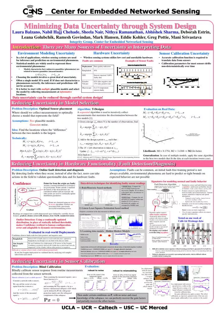
1. Injected CONSTANT fault In a deployment with all sensors in a styrofoam box, thus with a 1-d signal subspace, the algorithm recovers the gains and offsets almost exactly. Then assuming the measured signals y are a linear function of x: and assuming the true signals x lie in a known r-dimensional subspace of Rn which can be defined by P, the orthogonal projection matrix onto the orthogonal complement of that subspace: robust to noise Error at 2% noise in the measured signal: Gain: <.01% Offset: <2.4% robust to mismodeling Error at 10% of the true signal outside of the assumed subspace: Gain: <1% Offset: <4% Center for Embedded Networked Sensing Minimizing Data Uncertainty through System Design Laura Balzano, Nabil Hajj Chehade, Sheela Nair, Nithya Ramanathan, Abhishek Sharma, Deborah Estrin, Leana Golubchik, Ramesh Govindan, Mark Hansen, Eddie Kohler, Greg Pottie, Mani Srivastava Integrity Group, Center for Embedded Networked Sensing Introduction: There are Many Sources of Uncertainty in Interpreting Data Hardware Uncertainty Environment Modeling Uncertainty Sensor Calibration Uncertainty • In a lot of applications, wireless sensing systems are used for inference and prediction on environmental phenomena. • Statistical models are widely used to represent these environmental phenomena: • Models characterize how unknown quantities (phenomena) are related to known quantities (measurements): • Choosing the models involves a great deal of uncertainty. • Often a single model M is used. If M does not characterize a phenomenon correctly, the inferences and predictions will not be accurate. • It is better to start with multipleplausible models and select the model by collecting measurements at informative locations. • Wireless sensing systems utilize low cost and unreliable hardware Faults are common Examples of Sensor Faults • Accurate calibration function is required to translate data from sensors • Calibration parameters for most sensors drifts non-deterministically over time Data uncertainty can be reduced through careful system design! Reducing Uncertainty in Model Selection Problem Description: Optimal Sensor placement Where should we collect measurements to optimally choose a model that represents the field? Assumptions: Two plausible models. Gaussian noise. Idea: Find the locations where the “difference” between the two models is the largest. Technically: Algorithm:T-Designs A sequentialalgorithm is used to iteratively collect measurements that maximize the discrimination between the two models [1]. Evaluation on Real Data: Likelihoods: M1 0.1754, M2  3.4368  M2 fits better. Generalization: In case of multiple models, apply the same algorithm to the best two models that fit the data at each iteration (worst case). [1] A.C. Atkinson and V.V. Fedorov. Optimal design: Experiments for discriminating betweenseveral models. Biometrika 62, 289-303, 1975. Reducing Uncertainty in Hardware Functionality (Fault Detection/Diagnosis) Problem Description: Online fault detection and diagnosis By detecting faults when they occur, instead of after the fact, users can take actions in the field to validate questionable data and fix hardware faults. Assumptions: Faults can be common, an initial fault-free training period is not always available, environmental phenomena are hard to predict so tight bounds on expected behavior are not possible Signatures for modeling normal and faulty behavior Confidence Data-driven techniques for identifying faulty sensor readings 1) Rule/Heuristic-based methods Points far from the origin are faulty Assume a normal distribution of distances for good points. Points outside 2 standard deviations of the mean distance are considered outliers and are rejected. All other points are used to continually update distribution parameters. Fault Detection Algorithm (adapted from Detecting Fraud In the Real World; Cahill, Lambert, Pinhiero, and Sun; 2000) • Summarize sensor and fault behaviors using a signature: multivariate probability density of features(Cahill, Lambert, Pinhiero, and Sun; 2000) • Features chosen to exploit differences between faulty and normal behavior. Current features summarize temporal and spatial information: • Temporal: actual reading, change between successive readings, voltage • Spatial: diff. from neighboring sensors. • Calculate score for new readings using log likelihood ratio: Higher scores are more suspicious. • Use of sensor signatures allows for sensor-specific fault detection. • SHORT Rule: Compute the rate of change between two successive samples. If it is above a threshold, this is an instance of SHORT fault. • NOISE Rule : Compute the std. deviation of samples within time window W. If it is above a threshold, the samples are corrupted by NOISE fault. Take Physical Sample New reading Calculate Features: Xt Sensor signature: St Fault signature: F Standard Deviation Replace Sensor update sensor sig. Calculate score Points are clustered using an online K-means algorithm. Clusters are associated with a previously successful remediating action update fault sig. SHORT fault NOISE fault Score > threshold? NO 2) Linear-Least Squares Estimation based method • Exploits correlation in the data measured at different sensors • LLSE Equation: YES Gradient Signature update requires online density estimation • Sequentially update density estimate with each new reading • Unable to store historical data • Must compactly represent density • No single parametric family flexible enough to represent all distributions of features Developing a new method to do this using log-splines. Readings are mapped into a multi-dimensional space defined by carefully chosen features: gradient, distance from LDR, distance from NLDR, standard deviation. Tested on one week of Cold-Air Drainage data Outlier Detection: Using a continually updated distribution, in place of statically defined thresholds, makes Confidence resilient to human configuration error and adaptable to dynamic environments Low voltage 3) Learning data models : Hidden Markov Models Evaluated in real-world Deployments Confidence detects faults with low false positive and negative rates. Difficult to validate what is truly a fault without ground truth In our San Joaquin deployment we validated data by analyzing soil samples taken from each sensor • HMM model: • Number of states • Transition probabilities • Conditional probability: Pr [O | S ] Sensor 1 Sensor 2 stuck-at fault unusually noisy readings Sensor 2 malfunctioning at start of deployment; Noisy readings are learned as “normal” sensor behavior Results • Analyzed data sets from real world deployments to characterize the prevalence of data faults using these 3 methods. • NAMOS deployment : CONSTANT+NOISE faults, up to 30% of samples affected by data faults. • Intel Lab, Berkeley deployment: CONSTANT+NOISE faults, up to 20% of samples affected by data faults. • Great Duck Island deployment: SHORT+NOISE faults, 10-15% of samples affected by data faults. • SensorScope deployment: SHORT faults, very few samples affected by data faults. 4/06 4/08 4/10 4/12 • Difficult to initialize sensor signature without learning period that is guaranteed to be fault-free. • Can use a stricter threshold during learning period to decrease chance of incorporating faults into sensor signature • Method is dependent on accurately representing fault models, which is difficult without available labeled training data. Reducing Uncertainty in Sensor Calibration Evaluation: Problem Description: Blind Calibration Blindly calibrate sensor response from routine measurements collected from the sensor network. Manual calibration is not a scalable practice! Consider a network with n sensors. We can call the vector of a true signal from the n sensors x: And the vector of the measured signal y: In a deployment with sensors spread across a valley at the James Reserve, using a 4-d signal subspace constructed from the calibrated data, the gain calibration was quite accurate. The offset calibration, as expected, captured some of the non-zero mean signal; additionally it was sensitive to the model. Then under certain conditions on P, with no noise and exact knowledge of the subspace, we can perfectly recover the gain factors and partially recover the offset factors. UCLA – UCR – Caltech – USC – UC Merced