Download
1 / 6
60 likes | 236 Views
Predicting Future. Two Approaches to Predition. Extrapolation: Use past experiences for predicting future. One looks for patterns over time. Predictive models: Observed relationship between dependent and independent factors. Goodness of fit: estimated by analysis of residuals. .

E N D
Two Approaches to Predition • Extrapolation: Use past experiences for predicting future. One looks for patterns over time. • Predictive models: Observed relationship between dependent and independent factors. • Goodness of fit: estimated by analysis of residuals.
Commonly Used Methods • Bivariate Regression/simple regression. • Y=a+bx • Multiple Regression. • Y=a+b1x1+b2x2+b3x3+…+dnxn • Time Series Analysis • y=a+bt
Bivariate Regression • y=a+bx • A ‘least square’ criteria produces the lowest residual. • It is a test of linear association and not a test of causal relationship. • Should not be used to prediction outside the bounds of the data used.
Multiple Regression • Y=a+b1x1+b2x2+b3x3+…+dnxn • Special Cases: • Use of Dummy Variable (0 and 1 option as in nominal scale) • Use of standardized betas to compare the importance of independent variables. • Using Multiple Regression as a screening device. • Stepwise Regression.
Time Series Analysis • y=a+bt • Simple trend. • Exponential Smoothing. • F(t+1) = GXt+(1-G)Ft • Moving Averages. • F(t+1) = {Xt - X(t-N) }/N + Ft • Cycle and Seasonality Where: • F= forecast for the period. • X= actual value at a time. • N= number of values included in average, and • G=exponential smoothing parameter (gamma) and 0<=G<=1