Download
1 / 51
560 likes | 709 Views
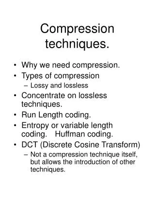
Chapter 10 Basic Video Compression Techniques. 10.1 Introduction to Video Compression 10.2 Video Compression with Motion Compensation 10.3 Search for Motion Vectors 10.4 H.261 10.5 H.263 10.6 Further Exploration. 10.1 Introduction to Video Compression.

E N D
Chapter 10Basic Video Compression Techniques 10.1 Introduction to Video Compression 10.2 Video Compression with Motion Compensation 10.3 Search for Motion Vectors 10.4 H.261 10.5 H.263 10.6 Further Exploration Li & Drew
10.1 Introduction to Video Compression • A video consists of a time-ordered sequence of frames, i.e., images. • An obvious solution to video compression would be predictive coding based on previous frames. Compression proceeds by subtracting images: subtract in time order and code the residual error. • It can be done even better by searching for just the right parts of the image to subtract from the previous frame. Li & Drew
10.2 Video Compression with Motion Compensation • Consecutive frames in a video are similar — temporal redundancy exists. • Temporal redundancy is exploited so that not every frame of the video needs to be coded independently as a new image. • The difference between the current frame and other frame(s) in the sequence will be coded — small values and low entropy, good for compression. • Steps of Video compression based on Motion Compensation (MC): 1. Motion Estimation (motion vector search). 2. MC-based Prediction. 3. Derivation of the prediction error, i.e., the difference. Li & Drew
Motion Compensation • Each image is divided into macroblocksof size NxN. • - By default, N= 16 for luminance images. For chrominance images, N= 8 if 4:2:0 chromasubsampling is adopted. • Motion compensation is performed at the macroblock level. • - The current image frame is referred to as Target Frame. • - A match is sought between the macroblock in the Target Frame and the most similar macroblock in previous and/or future frame(s) (referred to as Reference frame(s)). • - The displacement of the reference macroblock to the target macroblock is called a motion vector MV. • - Figure 10.1 shows the case of forward prediction in which the Reference frame is taken to be a previous frame. Li & Drew
MV search is usually limited to a small immediate neighborhood — both horizontal and vertical displacements in the range [−p, p]. This makes a search window of size (2p+ 1) x (2p+ 1). Fig. 10.1: Macroblocks and Motion Vector in Video Compression. Li & Drew
10.3 Search for Motion Vectors • The difference between two macroblocks can then be measured by their Mean Absolute Difference (MAD): (10.1) N—size of the macroblock, kandl — indices for pixels in the macroblock, iandj— horizontal and vertical displacements, C ( x + k, y + l ) — pixels in macroblock in Target frame, R ( x + i+ k, y + j + l ) — pixels in macroblock in Reference frame. • The goal of the search is to find a vector (i, j) as the motion vector MV = (u, v), such that MAD(i, j) is minimum: (10.2) Li & Drew
Sequential Search • Sequential search: sequentially search the whole (2p+ 1) x (2p+ 1) window in the Reference frame (also referred to as Full search). • a macroblock centered at each of the positions within the window is compared to the macroblock in the Target frame pixel by pixel and their respective MAD is then derived using Eq. (10.1). • The vector (i, j) that offers the least MADis designated as the MV (u, v) for the macroblock in the Target frame. • - sequential search method is very costly — assuming each pixel comparison requires three operations (subtraction, absolute value, addition), the cost for obtaining a motion vector for a single macroblock is (2p+ 1) (2p+ 1) N2 3 O ( p2 N2 ). Li & Drew
PROCEDURE 10.1 Motion-vector:sequential-search begin min_MAD= LARGE NUMBER; /* Initialization */ for i= −p to p for j = −p to p { cur_MAD= MAD(i, j); if cur_MAD < min_MAD { min_MAD= cur_MAD; u = i; /* Get the coordinates for MV. */ v = j; } } end Li & Drew
2D Logarithmic Search • Logarithmic search: a cheaper version, that is suboptimal but still usually effective. • The procedure for 2D Logarithmic Search of motion vectors takes several iterations and is akin to a binary search: • - As illustrated in Fig.10.2, initially only nine locations in the search window are used as seeds for a MAD-based search; they are marked as ‘1’. • - After the one that yields the minimum MADis located, the center of the new search region is moved to it and the step-size (“offset”) is reduced to half. • - In the next iteration, the nine new locations are marked as ‘2’ and so on. Li & Drew
Fig. 10.2: 2D Logarithmic Search for Motion Vectors. Li & Drew
PROCEDURE 10.2 Motion-vector:2D-logarithmic-search begin offset = ; Specify nine macroblocks within the search window in the Reference frame, they are centered at (x0,y0) and separated by offset horizontally and/or vertically; while last ≠ TRUE { Find one of the nine specified macroblocks that yields minimum MAD; if offset = 1 then last = TRUE; offset = offset/2 ; Form a search region with the new offset and new center found; } end Li & Drew
Using the same example as in the previous subsection, the total operations per second is dropped to: Li & Drew
Hierarchical Search • The search can benefit from a hierarchical (multiresolution) approach in which initial estimation of the motion vector can be obtained from images with a significantly reduced resolution. • Figure 10.3: a three-level hierarchical search in which the original image is at Level 0, images at Levels 1 and 2 are obtained by down-sampling from the previous levels by a factor of 2, and the initial search is conducted at Level 2. Since the size of the macroblock is smaller and pcan also be proportionally reduced, the number of operations required is greatly reduced. Li & Drew
Fig. 10.3: A Three-level Hierarchical Search for Motion Vectors. Li & Drew
Hierarchical Search (Cont'd) • Given the estimated motion vector (uk, vk) at Level k, a 3 x 3 neighborhood centered at (2 ·uk, 2 ·vk) at Level k − 1 is searched for the refined motion vector. • the refinement is such that at Level k − 1 the motion vector (uk−1 , vk−1) satisfies: • (2uk − 1 ≤ uk−1 ≤ 2uk +1, 2vk − 1 ≤ vk−1 ≤ 2vk +1) • Let (xk0, yk0) denote the center of the macroblock at Level kin the Target frame. The procedure for hierarchical motion vector search for the macroblock centered at (x00, y00) in the Target frame can be outlined as follows: Li & Drew
PROCEDURE 10.3 Motion-vector:hierarchical-search begin // Get macroblock center position at the lowest resolution Level k xk0 = x00 /2k ;yk0 = y00 /2k; Use Sequential (or 2D Logarithmic) search method to get initial estimated MV(uk, vk) at Level k; • while last ≠ TRUE { Find one of the nine macroblocks that yields minimum MADat Level k − 1 centered at • ( 2(xk0+uk) − 1 ≤ x ≤2(xk0+uk) + 1; 2(yk0 +vk) − 1 ≤ y ≤2(yk0+vk) + 1 ); if k = 1 then last = TRUE; k = k − 1; Assign (xk0; yk0 ) and (uk, vk) with the new center location and MV; } end Li & Drew
Table 10.1 Comparison of Computational Cost of MotionVector Search based on examples Li & Drew
10.4 H.261 • H.261: An earlier digital video compression standard, its principle of MC-based compression is retained in all later video compression standards. • - The standard was designed for videophone, video conferencing and other audiovisual services over ISDN. • - The video codec supports bit-rates of px64 kbps, where p ranges from 1 to 30 (Hence also known as p * 64). • - Require that the delay of the video encoder be less than 150 msec so that the video can be used for real-time bidirectional video conferencing. Li & Drew
ITU Recommendations & H.261 Video Formats • H.261 belongs to the following set of ITU recommendations for visual telephony systems: • H.221 — Frame structure for an audiovisual channel supporting 64 to 1,920 kbps. • H.230 — Frame control signals for audiovisual systems. • H.242 — Audiovisual communication protocols. • H.261 — Video encoder/decoder for audiovisual services at px64 kbps. • H.320 — Narrow-band audiovisual terminal equipment for px64 kbps transmission. Li & Drew
Fig. 10.4: H.261 Frame Sequence. Li & Drew
H.261 Frame Sequence • Two types of image frames are defined: Intra-frames (I-frames) and Inter-frames (P-frames): • - I-frames are treated as independent images. Transform coding method similar to JPEG is applied within each I-frame, hence “Intra”. • - P-frames are not independent: coded by a forward predictive coding method (prediction from a previous P-frame is allowed — not just from a previous I-frame). • - Temporal redundancy removal is included in P-frame coding, whereas I-frame coding performs only spatial redundancy removal. • To avoid propagation of coding errors, an I-frame is usually sent a couple of times in each second of the video. • Motion vectors in H.261 are always measured in units of full pixel and they have a limited range of ± 15 pixels, i.e., p= 15. Li & Drew
Intra-frame (I-frame) Coding Fig. 10.5: I-frame Coding. • Macroblocksare of size 16 x 16 pixels for the Y frame, and 8 x8 for Cb and Cr frames, since 4:2:0 chromasubsampling is employed. A macroblock consists of four Y, one Cb, and one Cr 8 x 8 blocks. • For each 8 x8 block a DCT transform is applied, the DCT coefficients then go through quantization zigzag scan and entropy coding. Li & Drew
Inter-frame (P-frame) Predictive Coding • Figure 10.6 shows the H.261 P-frame coding scheme based on motion compensation: • - For each macroblock in the Target frame, a motion vector is allocated by one of the search methods discussed earlier. • - After the prediction, a difference macroblockis derived to measure the prediction error. • - Each of these 8 x 8 blocks go through DCT, quantization, zigzag scan and entropy coding procedures. Li & Drew
The P-frame coding encodes the difference macroblock (not the Target macroblock itself). • Sometimes, a good match cannot be found, i.e., the prediction error exceeds a certain acceptable level. • - The MB itself is then encoded (treated as an Intra MB) and in this case it is termed a non-motion compensated MB. • For a motion vector, the differenceMVD is sent for entropy coding: MVD = MVPreceding− MVCurrent(10.3) Li & Drew
Fig. 10.6: H.261 P-frame Coding Based on Motion Compensation. Li & Drew
Quantization in H.261 • The quantization in H.261 uses a constant step_size, for all DCT coefficients within a macroblock. • If we use DCT and QDCT to denote the DCT coefficients before and after the quantization, then for DC coefficients in Intra mode: for all other coefficients: scale— an integer in the range of [1, 31]. (10.4) (10.5) Li & Drew
H.261 Encoder and Decoder • Fig. 10.7 shows a relatively complete picture of how the H.261 encoder and decoder work. • A scenario is used where frames I, P1, and P2 are encoded and then decoded. • Note: decoded frames (not the original frames) are used as reference frames in motion estimation. • The data that goes through the observation points indicated by the circled numbers are summarized in Tables 10.3 and 10.4. Li & Drew
Fig. 10.7: H.261 Encoder and Decoder. Li & Drew
Table 10.3: Data Flow at the Observation Points in H.261 Encoder Table 10.4: Data Flow at the Observation Points in H.261 Decoder Li & Drew
A Glance at Syntax of H.261 Video Bitstream • Fig. 10.8 shows the syntax of H.261 video bitstream: a hierarchy of four layers: Picture, Group of Blocks (GOB), Macroblock, and Block. • The Picture layer: PSC (Picture Start Code) delineates boundaries between pictures. TR (Temporal Reference) provides a time-stamp for the picture. • The GOB layer: H.261 pictures are divided into regions of 11 x 3 macroblocks, each of which is called a Group of Blocks (GOB). • Fig. 10.9 depicts the arrangement of GOBs in a CIF or QCIF luminance image. • For instance, the CIF image has 2 x 6 GOBs, corresponding to its image resolution of 352 x 288 pixels. Each GOB has its Start Code (GBSC) and Group number (GN). Li & Drew
In case a network error causes a bit error or the loss of some bits, H.261 video can be recovered and resynchronized at the next identifiable GOB. • GQuant indicates the Quantizer to be used in the GOB unless it is overridden by any subsequent MQuant (Quantizer for Macroblock). GQuant and MQuant are referred to as scalein Eq. (10.5). • The Macroblock layer: Each Macroblock (MB) has its own Address indicating its position within the GOB, Quantizer (MQuant), and six 8 x 8 image blocks (4 Y, 1 Cb, 1 Cr). • The Block layer: For each 8 x 8 block, the bitstream starts with DC value, followed by pairs of length of zerorun (Run) and the subsequent non-zero value (Level) for ACs, and finally the End of Block (EOB) code. The range of Run is [0; 63]. Level reflects quantized values — its range is [−127, 127] and Level ≠ 0. Li & Drew
Fig. 10.9: Arrangement of GOBs in H.261 Luminance Images. Li & Drew
10.5 H.263 • H.263 is an improved video coding standard for video conferencing and other audiovisual services transmitted on Public Switched Telephone Networks (PSTN). • Aims at low bit-rate communications at bit-rates of less than 64 kbps. • Uses predictive coding for inter-frames to reduce temporal redundancy and transform coding for the remaining signal to reduce spatial redundancy (for both Intra-frames and inter-frame prediction). Li & Drew
H.263 & Group of Blocks (GOB) • As in H.261, H.263 standard also supports the notion of Group of Blocks (GOB). • The difference is that GOBs in H.263 do not have a fixed size, and they always start and end at the left and right borders of the picture. • As shown in Fig. 10.10, each QCIF luminance image consists of 9 GOBs and each GOB has 11 x 1 MBs (176 x 16 pixels), whereas each 4CIF luminance image consists of 18 GOBs and each GOB has 44 x 2 MBs (704 x 32 pixels). Li & Drew
Fig. 10.10 Arrangement of GOBs in H.263 Luminance Images. Li & Drew
Motion Compensation in H.263 • The horizontal and vertical components of the MVare predicted from the median values of the horizontal and vertical components, respectively, of MV1, MV2, MV3 from the “previous”, “above” and “above and right” MBs (see Fig. 10.11 (a)). • For the Macroblock with MV(u, v): up= median(u1, u2, u3), vp= median(v1, v2, v3). (10.6) • Instead of coding the MV(u, v) itself, the error vector (δu, δv) is coded, where δu = u − upand δv = v − vp. Li & Drew
Half-Pixel Precision • In order to reduce the prediction error, half-pixel precision is supported in H.263 vs. full-pixel precision only in H.261. • - The default range for both the horizontal and vertical components uand vof MV(u, v) are now [−16, 15.5]. • - The pixel values needed at half-pixel positions are generated by a simple bilinear interpolation method, as shown in Fig. 10.12. Li & Drew
Fig. 10.12: Half-pixel Prediction by Bilinear Interpolation in H.263. Li & Drew
Optional H.263 Coding Modes • H.263 species many negotiable coding options in its various Annexes. Four of the common options are as follows: 1. Unrestricted motion vector mode: • - The pixels referenced are no longer restricted to be within the boundary of the image. • - When the motion vector points outside the image boundary, the value of the boundary pixel that is geometrically closest to the referenced pixel is used. • - The maximum range of motion vectors is [-31.5, 31.5]. Li & Drew
2. Syntax-based arithmetic coding mode: • - As in H.261, variable length coding (VLC) is used in H.263 as a default coding method for the DCT coefficients. • - Similar to H.261, the syntax of H.263 is also structured as a hierarchy of four layers. Each layer is coded using a combination of fixed length code and variable length code. 3. Advanced prediction mode: • - In this mode, the macroblock size for MC is reduced from 16 to 8. • - Four motion vectors (from each of the 8 x 8 blocks) are generated for each macroblock in the luminance image. Li & Drew
4. PB-frames mode: • - In H.263, a PB-frame consists of two pictures being coded as one unit, as shown Fig. 10.13. • - The use of the PB-frames mode is indicated in PTYPE. • - The PB-frames mode yields satisfactory results for videos with moderate motions. • - Under large motions, PB-frames do not compress as well as B-frames and an improved new mode has been developed in Version 2 of H.263. Li & Drew
Fig. 10.13: A PB-frame in H.263. Li & Drew
H.263+ and H.263++ • The aim of H.263+: broaden the potential applications and offer additional flexibility in terms of custom source formats, different pixel aspect ratio and clock frequencies. • H.263+ provides 12 new negotiable modes in addition to the four optional modes in H.263. • - It uses Reversible Variable Length Coding (RVLC) to encode the difference motion vectors. • - A slice structure is used to replace GOB to offer additional flexibility. Li & Drew
- H.263+ implements Temporal, SNR, and Spatial scalabilities. • - Support of Improved PB-frames mode in which the two motion vectors of the B-frame do not have to be derived from the forward motion vector of the P-frame as in Version 1. • - H.263+ includes deblocking filters in the coding loop to reduce blocking effects. Li & Drew
H.263++ includes the baseline coding methods of H.263 and additional recommendations for Enhanced Reference Picture Selection (ERPS), Data Partition Slice (DPS), and Additional Supplemental Enhancement Information. • - The ERPS mode operates by managing a multi-frame buffer for stored frames — enhances coding efficiency and error resilience capabilities. • - The DPS mode provides additional enhancement to error resilience by separating header and motion vector data from DCT coefficient data in the bitstream and protects the motion vector data by using a reversible code. Li & Drew