Download
1 / 48
480 likes | 603 Views
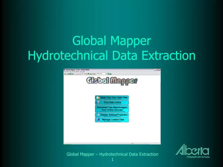
Global Mapper Hydrotechnical Data Extraction. Overview. Projection Drainage Area Stream Profile XS Data. Projection.

E N D
Overview • Projection • Drainage Area • Stream Profile • XS Data
Projection • Most measurement applications in Global Mapper look and work better if the projection is set to a Transverse Mercator projection, where one metre will look the same in both the North-South and East-West directions. • Options for Alberta include UTM Zone 11 (W of 114deg), UTM Zone 12 (E of 114 deg), 10TM (entire province) or 3TM (smaller areas, e.g. survey). • Different GIS data files may store data in different projection systems, but Global Mapper will convert and display in the selected projection. • To select projection – Tools: Configuration (or Configuration button), select “Projection Tab”, pick from list for UTM, “Load From File” for 10TM or 3TM (point to root of GIS folder, pick PRJ file).
Drainage Area (DA) - Overview • Locate Map Sheet number for Site • Open Global Mapper and set projection to a TM type • Load GIS Data - DEM, Streams, and Bridges (photos, lidar etc.) • Zoom to extents of DA • Generate Contours • Draw DA boundary • Modify DA, if necessary • Large DA – Use Multiple Polygons
1. Locate Map Sheet Number • Use HIS to locate Map Sheet Number for Bridge Site
2. Open Global Mapper • Open Global Mapper and Set Projection to TM type
3a. Load GIS Data - DEM • Drag and drop DEM file from GIS folder (DEM\83B\83B16.bil)
3b. Load GIS Data - Streams • Drag and drop Stream file from GIS folder (Streams\83B Streams.zip)
3c. Load GIS Data - Bridges • Drag and drop Bridges file from GIS folder (Bridges.zip)
4. Zoom to Extents of DA • Find selected site (centre) • Zoom in/out to extent of DA – use DEM and Streams as guide • Add additional DEM and Streams files as necessary • Refine zoom, if necessary, with zoom tool
4a. Find Bridge Site • Search : “Search By Name” • Enter Site Number • Double click on number on list • Click OK - bridge will now be in the centre of the screen Type Here Double Click Here
4b. Zoom In/Out • Use Zoom, Zoom In, Zoom Out, and Pan tools to zoom to visible extents of DA, with DEM and streams as rough guide.
4c. Add more DEM, Streams • If necessary, add additional DEM and Streams layers to cover the entire DA
4d. Refine Zoom • If necessary, add additional DEM and Streams layers to cover the entire DA
5. Generate Contours • File : Generate Contours Select this to limit contouring to screen area, much faster than “all loaded data” Enter Contour Interval e.g. 10m for steep areas, 2m for flat areas
6. Draw DA Boundary • Select Measure Tool • Start clicking at outlet point, click points along DA boundary : • Follow ridge lines in the contours • Include all stream tributaries • Cross contours on square • hold down “Alt” key to avoid snapping to elements • Note DA on status bar before closing polygon • Close polygon by right clicking on outlet point (select “Save Measurement” to keep measurement as area or line) • Area – retains measurement but shades polygon display and can interfere with selecting features • Line – does not retain measurement, but can be converted to an Area feature later, if necessary
6b. Draw DA Boundary Measurement in progress
6c. Draw DA Boundary Outlet Point Area Measurement
7. Modify DA Boundary • Zoom to area of interest • Turn on “Render Vertices” – Shift + V • Select point to be moved • Right-click on point and select “Move Selected Vertex” (or Alt + click) • Move point to desired location • Points can also be inserted and deleted • Area – retains measurement but shades polygon display and can interfere with selecting features • Line – does not retain measurement, but can be converted to an Area feature later, if necessary
7. Modify DA Boundary • If edited polygon is an Area shape, the area measurement will be automatically updated (double click with digitizer tool or click with Info tool to see updated value). • If polygon is a Line shape, the following steps are required to see the updated area: • Select Line • Right click and select “Create New Area Feature from Selected Line” • Right click on new Area shape and select “Add/Update the Measure Attributes of Selected Feature” • Read area value the same way as for an Area shape (see above)
7. Modify DA Boundary Selected Vertex
7. Modify DA Boundary Points moved, inserted
8. Multiple Polygons • For large DA’s that can’t be easily analysed on one screen, multiple polygons can be used as follows: • Identify recognizable points for which incremental areas can be assessed on one screen at a reasonable level of zoom (e.g. bridges, confluences, other features on imagery…) • Measure the DA for the most upstream point. • Add an incremental measurement for each subsequent downstream point, using previous DA boundary as a guide for common boundaries (don’t hold down Alt key to snap) • Sum DA’s for all polygons to get total • A similar process can be used to break basins into sub-basins for qualitative assessment of runoff or quantitative routing calculations.
Stream Profile - Overview • Starting with file for DA, prepare for stream selection • Select all arcs that make up the stream • Combine Arcs to form one line • Generate Profile for line • Calculate slope for desired location • (Optional - HIS Only) Import profile into HIS
1. Prepare for Stream Selection • Open Overlay Control Center • Un-check any vector layers that may affect stream arc selection: • especially “Generated Contours” layers • also “User Created Features” layer to hide DA polygons • can leave bridge points on as they won’t interfere with line selection • Zoom to extent of stream to be profiled
2. Select Stream Arcs - Unnamed • Unnamed streams – add arcs technique: • Select upstream arc using digitizer tool • Add the next downstream arc (CTRL + click) • Continue to end of stream • Unnamed streams – remove arcs technique: • Select all vectors in stream network by dragging a box with the digitizer tool • Remove arcs that are not on the main stream (SHFT + click)
2. Select Stream Arcs - Named • Search – Search By Name – enter part of stream name • In list, click on 1st match item, SHFT + click on last match item • Click “Edit Selected”, “Create New Type”, enter name (OK-OK-Close) • Configuration – Vector Display Tab – Filter Lines – Clear All and click check box by new feature (OK-OK) • Draw box around all remaining contiguous arcs on screen
2. Stream Selection - Named Enter start of Stream name Click here to create new type Select all matches Click here to set type
2. Stream Selection - Named Click here to turn off all lines Click here to turn off other lines Click here to turn on new line type
2. Stream Selection - Named Selected Stream
3. Combine Selected Arcs • Right Click on selected arcs and click on “Combine Selected Line Features” and “OK” • De-select and re-select line to make sure all arcs were combined. If not, turn on “Render Vertices (SHFT + V)” and zoom in at points where the line combination failed and fix the problem by: • If lines are not contiguous - connect the lines with a short arc or snap move one vertex on top of the other • If the wrong arc was selected (such as a tributary), break that line at the confluence point and re-select and combine on the correct line. • Once lines are combined, they will be moved from the active Streams layer to the “User Created Feature” layer, and may disappear if this layer is hidden.
4. Generate Profile • Right Click on the combined line segment and click on “Generate Path Profile Along Line”. This option will not appear if a DTM layer is not turned on. • A plot of the profile of the line will appear
5. Calculate Slope at Point • Estimate Slope from Plot • Identify approximate station of point of interest along profile (measure if necessary) • Identify which profile section applies to this point (if point is near cusp of 2 significantly different slope sections, more work will be required to estimate slope. • Identify the coordinates of 2 points on the appropriate slope section and calculate slope as dy/dx. • Export Data to Spreadsheet and calculate Slope • From Plot window, select File – Save Distance/Elevation File • Open saved file in spreadsheet • Plot as necessary and calculate slope between 2 points defining slope for point of interest
6. Import to HIS • Export Data to x,y,z text file • Change projection temporarily to Geographic • From Plot window, select File – Save XYZ File as xxxx.xyz where xxxx = unique ID code for this stream used by HIS • Save XYZ files for other streams as necessary • Import into “Stream Slopes.mdb” File • Open “Add Prof to DB” tool • Enter stream ID numbers to add and point to path of exported files and click “Go” • The stream profile will now be available within HIS, allowing precise locating of the bridge on the profile and the use of the built-in slope calculation tool.
XS Data • DTM – XS Extraction • Imagery Measurement
1. DTM - XS Extraction • Open DTM layer: • 100m spacing DTM generally insufficient for XS (B,h,T) • Better - LIDAR, Photogrammetry, 3D surfaces from survey points • Identify XS locations that appear to be typical of the channel (see Hydrotechnical Design Guidelines) • View Elevation Profile: • Use 3D Path Tool to draw the line to be profiled (good for quick views, but line will not be saved) • Use Measure Tool or Digitizer Tool to draw line and save as line when done. Right click on saved line and select “Generate Path Profile Along Line” • Characterize typical values for B, h, and T based on the profile plots at selected sections (export to text file for use in other tools, if necessary).
1. DTM – XS Extraction LIDAR 100m DTM
1. DTM – XS Extraction LIDAR 100m DTM
2. Imagery Measurement • Open Imagery layer: • Satellite imagery OK for large rivers but too grainy (2.5m pixels) for small channels when zoomed in • Georeferenced airphotos allow for more precise scaling • Identify XS locations that appear to be typical of the channel (see Hydrotechnical Design Guidelines) • Use Measure Tool to measure channel dimensions at selected locations: • B - based largely on water surface width or width between vegetation • T – based on visual clues as to top of bank (apparent elevation change, change in vegetation) • h – difficult to assess from imagery. Visual comparison with other sites where ‘h’ is known will help to set limits on bank height. • Characterize typical values for B and T based on the measurements
2. Imagery Measurement Satellite Image
2. Imagery Measurement Georeferenced Airphoto