A Field Guide to Genetic Programming

1. John R. Koza [Edited by J. Wiebe]

2. GENETIC PROGRAMMING

3. Notes • [added by J. Wiebe] • A Field Guide to Genetic Programming, 2008, Poli, Langdon, McPhee, Koza (easy to find via Google) • Author of these slides, John Koza, is a pioneer in the field

4. THE CHALLENGE "How can computers learn to solve problems without being explicitly programmed? In other words, how can computers be made to do what is needed to be done, without being told exactly how to do it?"  Attributed to Arthur Samuel (1959)

5. CRITERION FOR SUCCESS "The aim [is] ... to get machines to exhibit behavior, which if done by humans, would be assumed to involve the use of intelligence.“  Arthur Samuel (1983)

6. Decision trees If-then production rules Horn clauses Neural nets Bayesian networks Frames Propositional logic Binary decision diagrams Formal grammars Coefficients for polynomials Reinforcement learning tables Conceptual clusters Classifier systems REPRESENTATIONS

7. GENETIC PROGRAMMING (GP) • GP applies the approach of the genetic algorithm to the space of possible computer programs • Computer programs are the lingua franca for expressing the solutions to a wide variety of problems • A wide variety of seemingly different problems from many different fields can be reformulated as a search for a computer program to solve the problem.

8. GP FLOWCHART

9. A COMPUTER PROGRAM IN C int foo (int time) { int temp1, temp2; if (time > 10) temp1 = 3; else temp1 = 4; temp2 = temp1 + 1 + 2; return (temp2); }

10. PROGRAM TREE (+ 1 2 (IF (> TIME 10) 3 4))

11. CREATING RANDOM PROGRAMS

12. CREATING RANDOM PROGRAMS • Available functions F = {+, -, *, %, IFLTE} • Available terminals T = {X, Y, Random-Constants} • The random programs are: • Of different sizes and shapes • Syntactically valid • Executable

13. GP GENETIC OPERATIONS • Reproduction • Mutation • Crossover • Architecture-altering operations

14. MUTATION OPERATION • Select 1 parent probabilistically based on fitness • Pick point from 1 to NUMBER-OF-POINTS • Delete subtree at the picked point • Grow new subtree at the mutation point in same way as generated trees for initial random population (generation 0) • The result is a syntactically valid executable program • Put the offspring into the next generation of the population • [Example: in class]

15. CROSSOVER OPERATION • Select 2 parents probabilistically based on fitness • Randomly pick a number from 1 to NUMBER-OF-POINTS for 1st parent • Independently randomly pick a number for 2nd parent • The result is a syntactically valid executable program • Put the offspring into the next generation of the population • Identify the subtrees rooted at the two picked points • [Example in class]

16. REPRODUCTION OPERATION • Select parent probabilistically based on fitness • Copy it (unchanged) into the next generation of the population

17. [Initialization] • Maximum initial depth of tree Dmax is set • Full method (each branch has depth = Dmax): • nodes at depth d < Dmax randomly chosen from function set F • nodes at depth d = Dmax randomly chosen from terminal set T • Grow method (each branch has depth  Dmax): • nodes at depth d < Dmax randomly chosen from F  T • nodes at depth d = Dmax randomly chosen from T • Common GP initialisation: ramped half-and-half, where grow & full method each deliver half of initial population • Ramped: use a range of depth limits

18. [Pseudocode for program generationmethod is either ‘full’ or ‘grow’] Gen(max_d, method) • If max_d = 0 or (method = grow and rand[0,1] < |term_set| / (|term_set|+|func_set|)) then • Expr = random(term_set) • Else • Func = random(func_set) • For i = 1 to arity(func): • Arg_i = Gen(max_d – 1, method) • Expr = (Func, arg_1, arg_2, …) • Return Expr

19. Bloat • Bloat = “survival of the fattest”, i.e., the tree sizes in the population are increasing over time • Ongoing research and debate about the reasons • Needs countermeasures, e.g. • Prohibiting variation operators that would deliver “too big” children • Parsimony pressure: penalty for being oversized • [This will come up again later]

20. FIVE MAJOR PREPARATORY STEPS FOR GP • Determining the set of terminals • Determining the set of functions • Determining the fitness measure • Determining the parameters for the run • Determining the method for designating a result and the criterion for terminating a run

21. [Issues with function sets] • Typically, Closure is required • Type consistency – any subtree may be used in any argument position for every function • Why? Initial tree generation, subtree generation in mutation, and crossover may generate any combination. • Require that all functions argument and return types are the same • Seems limiting, but can often be gotten around • Subcase: allowed type conversions, such as boolean to int • Subcase: make function general; some uses will ignore things • Alternative: crossover and mutation constrained to produce only type compatible programs (Section 6.2 in the Field Guide)

22. [Issues with function sets] • Typically, Closure is required • 2. Evaluation safety • E.g. protected values of numeric functions. Instead of throwing an exception, return a default value. E.g., 4/0 returns 1. • E.g. no-ops in planning, such as move-forward when the robot is face forward against the wall

23. [Issues with Function Sets] • Type consistency and evaluation safety may go hand in hand • Suppose type T covers all the types we want to use. • Suppose a function’s arguments should only range over a subset of values covered by T • A protected version of the function returns a default value for arguments of types the function is not actually defined over.

24. [Issues with Function Sets] • Alternative to protected functions: trap run-time exceptions and strongly reduce the fitness of programs that generate such errors • But, this may introduce many “nonsense” individuals in the population, all with similar fitness. The GP system may not be able to “find” the valid individuals

25. Structures other than Programs • In design problems, the solution may be an artifact. Bridge, circuit, etc. Functions may build structures, rather than be computer code. (We may return to this later. Before that, we’ll assume solutions are computer code.)

26. [Fitness function] • E.g., error between output and the desired output; payoff, in a game-playing setting; compliance of a structure with design criteria • The fact that individuals are computer programs brings up a couple issues for evaluating fitness …

27. [Fitness function evaluation] • Not simply a function application, F(X) • X is a program • X needs to be executed • On multiple inputs • So, part of specifying the fitness evaluation is specifying which inputs • Computationally expensive: multiple executions of each member of the population • Compilation? Depending on the primitive set (the terminal and function sets), the overhead of building/testing a compiler might not be worth it. So, often, evaluation is via interpreter, even though more expensive

28. [Interpreter for a expr in prefix notation, represented as a list] • If expr is a list then • Proc = expr(1) • Val = proc(eval(expr(2)), eval(expr(3)), …) • Else • If expr is a variable or constant then • Val = expr • Else • Val = expr() {terminal 0-arity function: execute) • Return Val • Example in class

29. ILLUSTRATIVE GP RUN

30. SYMBOLIC REGRESSION

31. PREPARATORY STEPS

32. SYMBOLIC REGRESSION POPULATION OF 4 RANDOMLY CREATED INDIVIDUALS FOR GENERATION 0

33. x + 1 x2 + 1 2 x 4.4 6.0 9.48 15.4 SYMBOLIC REGRESSION x2 + x + 1 FITNESS OF THE 4 INDIVIDUALS IN GEN 0 [Note: I recalculated these values – these are the sums of the absolute vals of the differences between predicted values and Y values at the sample points; That’s the calculation you need to know.]

34. First offspring of crossover of (a) and (b)  picking “+” of parent (a) and left-most “x” of parent (b) as crossover points Second offspring of crossover of (a) and (b)  picking “+” of parent (a) and left-most “x” of parent (b) as crossover points Mutant of (c) picking “2” as mutation point Copy of (a) SYMBOLIC REGRESSION x2 + x + 1 GENERATION 1

35. CLASSIFICATION

36. GP TABLEAU – INTERTWINED SPIRALS

37. WALL-FOLLOWER

38. FITNESS

39. BEST OF GENERATION 57

40. BOX MOVER – BEST OF GEN 0

41. BOX MOVERGEN 45 – FITNESS CASE 1

42. TRUCK BACKER UPPER

43. TRUCK BACKER UPPER • 4-Dimensional control problem • horizontal position, x • vertical position, y • angle between trailer and horizontal, Qt • angle between trailer and cab, Qd • One control variable (steering wheel turn angle) • State transition equations map the 4 state variables into 1 output (the control variable) • Simulation run over many initial conditions and over hundreds of time steps

44. COMPUTER PROGRAMS • Subroutines provide one way to REUSE code  possibly with different instantiations of the dummy variables (formal parameters) • Loops (and iterations) provide a 2nd way to REUSE code • Recursion provide a 3rd way to REUSE code • Memory provides a 4th way to REUSE the results of executing code

45. DIFFERENCE IN VOLUMES D = L0W0H0 – L1W1H1

46. AUTOMATICALLY DEFINED FUNCTION volume

47. AUTOMATICALLY DEFINED FUNCTION volume (progn (defun volume (arg0 arg1 arg2) (values (* arg0 (* arg1 arg2)))) (values (- (volume L0 W0 H0) (volume L1 W1 H1))))

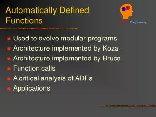
48. AUTOMATICALLY DEFINED FUNCTIONS • ADFs provide a way to REUSE code • Code is typically reused with different instantiations of the dummy variables (formal parameters)

49. ADF IMPLEMENTATION • Each overall program in population includes • a main result-producing branch (RPB) and • function-defining branch (i.e., automatically defined function, ADF) • In generation 0, create random programs with different ingredients for the RPB and the ADF • Terminal set for ADF typically contains dummy arguments (formal parameters), such as ARG0, ARG1, … • Function set of the RPB contains ADF0 • ADFs are private and associated with a particular individual program in the population

50. ADF MUTATION • Select parent probabilistically on the basis of fitness • Pick a mutation point from either RPB or an ADF • Delete sub-tree rooted at the picked point • Grow a new sub-tree at the picked point composed of the allowable ingredients appropriate for the picked point • The offspring is a syntactically valid executable program