Download

1 / 40
410 likes | 699 Views
EART162: PLANETARY INTERIORS. Francis Nimmo. Last week - Seismology. Seismic velocities tell us about interior properties. Adams-Williamson equation allows us to relate density directly to seismic velocities. Travel-time curves can be used to infer seismic velocities as a function of depth

E N D
EART162: PLANETARY INTERIORS Francis Nimmo
Last week - Seismology • Seismic velocities tell us about interior properties • Adams-Williamson equation allows us to relate density directly to seismic velocities • Travel-time curves can be used to infer seismic velocities as a function of depth • Midterm
This Week – Fluid Flow & Convection • Fluid flow and Navier-Stokes • Simple examples and scaling arguments • Post-glacial rebound • Rayleigh-Taylor instabilities • What is convection? • Rayleigh number and boundary layer thickness • See Turcotte and Schubert ch. 6
Viscosity • Young’s modulus gives the stress required to cause a given deformation (strain) – applies to a solid • Viscosity is the stress required to cause a given strain rate – applies to a fluid • Viscosity is basically the fluid’s resistance to flow viscous elastic viscosity Young’s modulus • Kinematic viscosity h measured in Pa s • [Dynamic viscosity n=h/r measured in m2s-1] • Typical values for viscosity: water 10-3 Pa s, basaltic lava 104 Pa s, ice near melting 1014 Pa s, mantle 1021 Pa s • Viscosity often temperature-dependent (see Week 3)
d a Defining Viscosity • Recall • Viscosity is the stress generated for a given strain rate • Example – moving plate: u (Shear) stress s required to generate velocity gradient u / d (= ) Viscosity h=s d / u h • Example – moving lava flow: Driving shear stress = rgd sinq Surface velocity = rgd2sinq / h d e.g. Hawaiian flow h=104 Pa s q=5od=3m gives u=2 ms-1 (walking pace) q
Adding in pressure • In 1D, shear stress (now using t) is • Let’s assume u only varies in the y direction Viscous force (x direction, per unit volume): Fluid velocity u y dy x Pressure force (x direction, per unit volume): dx Why the minus sign?
Putting it together • Total force/volume = viscous + pressure effects • We can use F=ma to derive the response to this force What does this mean? • So the 1D equation of motion in the x direction is What does each term represent? • In the y-direction, we would also have to add in buoyancy forces (due to gravity)
Navier-Stokes • We can write the general (3D) formula in a more compact form given below – the Navier-Stokes equation • The formula is really a mnemonic – it contains all the physics you’re likely to need in a single equation • The vector form given here is general (not just Cartesian) Yuk!Inertial term. Source of turbulence. See next slide. Pressure gradient Buoyancy force (e.g. thermal or electromagnetic) is a unit vector Diffusion-like viscosity term. Warning: is complicated, especially in non-Cartesian geom. Zero for steady- state flows
a Reynolds number • Is the inertial or viscousterm more important? • We can use a scaling argument to get the ratio Re: Here L is a characteristic lengthscale of the problem Re • Re is the Reynolds number and tells us whether a flow is turbulent (inertial forces dominate) or not • Fortunately, many geological situations allow us to neglect inertial forces (Re<<1) • E.g. what is Re for the convecting mantle?
a Example 1 – Channel Flow L y x u 0 2d • 2D channel, steady state, u=0 at y=+d and y=-d P2 P1 (Here u doesn’t vary in x-direction) • Max. velocity (at centreline) = (DP/L) d2/2h • Does this result make sense? • We could have derived a similar answer from a scaling argument – how?
a Example 2 – falling sphere r Steady-state. What are the important terms? h u An order of magnitude argument gives drag force ~ hur Is this dimensionally correct? The full answer is 6phur, first derived by George Stokes in 1851 (apparently under exam conditions) By balancing the drag force against the excess weight of the sphere (4pr3Drg/3 ) we can obtain the terminal velocity (here Dr is the density contrast between sphere and fluid)
a Example 3 – spreading flow h(x,t) y Low Re, roughly steady-state. What are the important terms? u d x Conservation of mass gives (why?) As long as d >>h, we get: What kind of equation is this? Does it make physical sense? Where might we apply it on Earth?
ice w L mantle a Postglacial Rebound • Postglacial rebound problem: How long does it take for the mantle to rebound? • Two approaches: • Scaling argument • Stream function j – see T&S mantle • Scaling argument: • Assume u is constant (steady flow) and that u ~ dw/dt • We end up with decay constant • What does this equation mean?
Prediction and Observations How does this time constant compare with that for spreading flow? • Scaling argument gives: Hudson’s Bay deglaciation: L~1000 km, t=2.6 ka So h~2x10²¹ Pa s So we can infer the viscosity of the mantle A longer wavelength load would sample the mantle to greater depths – higher viscosity http://www.geo.ucalgary.ca/~wu/TUDelft/Introduction.pdf
L l l u1 u1 b u2 Rayleigh-Taylor Instability b r1 m • This situation is gravitationally unstable if r2 < r1 : any infinitesimal perturbation will grow • What wavelength perturbation grows most rapidly? r2 m b • The full solution is v. complicated (see T&S 6-12) – so let’s try and think about it physically . . . L
a R-T Instability (cont’d) • Recall from Week 5: dissipation per unit volume • We have two contributions to total dissipation ( ) • By adding the two contributions, we get term term • What wavelength minimizes the dissipation? • We end up with dissipation minimized at lmin=1.26 b • This compares pretty well with the full answer (2.57b) and saves us about six pages of maths
R-T instability (cont’d) • The layer thickness determines which wavelength minimizes viscous dissipation • This wavelength is the one that will grow fastest • So surface features (wavelength) tell us something about the interior structure (layer thickness) Salt domes in S Iran. Dome spacing of ~15 km suggests salt layer thickness of ~5 km, in agreement with seismic observations ~50km
Convection Cold - dense Fluid • Convection arises because fluids expand and decrease in density when heated • The situation on the right is gravitationally unstable – hot fluid will tend to rise • But viscous forces oppose fluid motion, so there is a competition between viscous and (thermal) buoyancy forces Hot - less dense • So convection will only initiate if the buoyancy forces are big enough • What is the expression for thermal buoyancy forces?
Conductive heat transfer • Diffusion equation (1D, Cartesian) Heat production Advected component Conductive component • Thermal diffusivity k=k/rCp(m2s-1) • Diffusion timescale:
Convection equations • There are two: one controlling the evolution of temperature, the other the evolution of velocity • They are coupled because temperature affects flow (via buoyancy force) and flow affects temperature (via the advective term) Navier- Stokes Buoyancy force Note that here the N-S equation is neglecting the inertial term Thermal Evolution Advective term • It is this coupling that makes solving convection problems hard
a Initiation of Convection Top temperature T0 d • Recall buoyancy forces favour motion, viscous forces oppose it • Another way of looking at the problem is there are two competing timescales – what are they? Incipient upwelling d Hot layer Bottom temp. T1 • Whether or not convection occurs is governed by the dimensionless (Rayleigh) number Ra: • Convection only occurs if Ra is greater than the critical Rayleigh number, ~ 1000 (depends a bit on geometry)
Constant viscosity convection T0 (T0+T1)/2 cold T0 d • Convection results in hot and cold boundary layers and an isothermal interior • In constant-viscosity convection, top and bottom b.l. have same thickness Isothermal interior d d T1 hot T1 • Heat is conducted across boundary layers • In the absence of convection, heat flux • So convection gives higher heat fluxes than conduction • The Nusselt number defines the convective efficiency:
d d d a Boundary layer thickness • We can balance the timescale for conductive thickening of the cold boundary layer against the timescale for the cold blob to descend to obtain an expression for the b.l. thickness d: • So the boundary layer gets thinner as convection becomes more vigorous • Also note that d is independent of d. Why? • We can therefore calculate the convective heat flux:
Example - Earth • Does this equation make sense? • Plug in some parameters for the terrestrial mantle: r=3000 kg m-3, g=10 ms-2, a=3x10⁻⁵ K-1, k=10-6 m2s-1, h=3x10²¹ Pa s, k=3 W m-1K-1, (T1-T0) =1500 K • We get a convective heat flux of 170 mWm-2 • This is about a factor of 2 larger than the actual terrestrial heat flux (~80 mWm-2) – not bad! • NB for other planets (lacking plate tectonics), d tends to be bigger than these simple calculations would predict, and the convective heat flux smaller • Given the heat flux, we can calculate thermal evolution
Summary • Fluid dynamics can be applied to a wide variety of geophysical problems • Navier-Stokes equation describes fluid flow: • Post-glacial rebound timescale: • Behaviour of fluid during convection is determined by a single dimensionless number, the Rayleigh number Ra
End of lecture • Supplementary material follows
Thermodynamics & Adiabat • A packet of convecting material is often moving fast enough that it exchanges no energy with its surroundings • What factors control whether this is true? • As the convecting material rises, it will expand (due to reduced pressure) and thus do work (W = P dV) • This work must come from the internal energy of the material, so it cools • The resulting change in temperature as a function of pressure (dT/dP) is called an adiabat • Adiabats explain e.g. why mountains are cooler than valleys
Adiabatic Gradient (1) • If no energy is added or taken away, the entropy of the system stays constant • Entropy S is defined by Here dQ is the amount of energy added to the system (so if dQ=0, then dS=0 also and the system is adiabatic) • What we want is at constant S. How do we get it? • We need some definitions: Maxwell’s identity Specific heat capacity (at constant P) Thermal expansivity
a T Adiabatic Gradient (2) z • We can assemble these pieces to get the adiabatic temperature gradient: adiabat • NB You’re not going to be expected to reproduce the derivation, but you do need to learn the final result • An often more useful expression can be obtained by converting pressure to depth (how?) • What are typical values for terrestrial planets?
v(y) u(x) dy u(x+dx) If V1=V2then v(y+dy) a Incompressibility & Stream Function dx • In many fluids the total volume doesn’t change Incompressibility condition • We can set up a stream functionj which automatically satisfies incompressibility and describes both the horizontal and the vertical velocities: Note that these satisfy incompressibility
a Stream Function j • Only works in 2 dimensions • Its usefulness is we replace u,v with one variable j Check signs here! Differentiate LH eqn. w.r.t. z and RH w.r.t x The velocity field of any 2D viscous flow satisfies this equation
a Postglacial rebound and j (1) • Biharmonic equation for viscous fluid flow • Assume (why?)j is a periodic function j=sin kx Y(y) Here k is the wavenumber = 2p/l • After a bit of algebra, we get • All that is left (!) is to determine the constants which are set by the boundary conditions – in real problems, this is often the hardest bit • What are the boundary conditions? • u=0 at z=0, v=dw/dt at z=0, u=v=0 at large z
2 1 a a Postglacial rebound and j (2) • Applying the boundary conditions we get • We have dw/dt = : • Vert. viscous stress at surface (z=0) balances deformation: Why can we ignore this term? • For steady flow, we can derive P from Navier-Stokes • Finally, eliminating A from 1 and 2 we get (at last!): This ought to look familiar . . .
Postglacial rebound (concluded) • So we get exponential decay of topography, with a time constant depending on wavenumber (k) and viscosity (h) • Same result as we got with the scaling argument! • Relaxation time depends on wavelength of load • Relaxation time depends on viscosity of fluid
Convection Cold - dense Fluid • Convection arises because fluids expand and decrease in density when heated • The situation on the right is gravitationally unstable – hot fluid will tend to rise • But viscous forces oppose fluid motion, so there is a competition between viscous and (thermal) buoyancy forces Hot - less dense • So convection will only initiate if the buoyancy forces are big enough • Note that this is different to the Rayleigh-Taylor case: thermal buoyancy forces decay with time (diffusion), compositional ones don’t • What is the expression for thermal buoyancy forces?
THIS SECTION PROBABLY A WASTE OF TIME txy v txy y txx u 1 tyy a Two Dimensions . . . x • In 1D, shear stress (now using t) is • In 2D, there are three different stresses: Shear stress Normal stresses • Where do the factors of 2 come from? p(y)dx • Force due to pressure (x direction, per unit cross-sectional area): p(x)dy dy p(x+dx)dy dx p(y+dy)dx EXPLAIN WHERE –VE COMES FROM
1 2 2 a a Viscous forces on an element (1) x txy • Viscous force (x direction, per unit cross-sectional area): v txy y txx u dy • Total force balance given by viscous + pressure forces tyy dx + • After some algebra, we get total force in x-direction: Note that force in x-direction only depends on velocity in x-direction and the x-gradient of pressure
Viscous forces on an element (2) • In the y-direction, body forces can also be important • Otherwise, the analysis is the same as before • We can use F=ma to derive the response to this force What does this mean? • So the equations of motion in x and y directions are
Putting it together • x-direction • y-direction Pressure gradient Body force Viscous terms • Special cases: • Steady-state – Du/Dt=0 • One-dimension (e.g. v=0, u only varies in y direction)