Download
1 / 18
190 likes | 299 Views
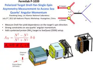
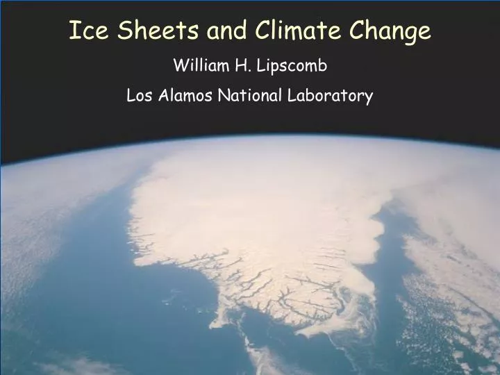
Ice Sheets and Climate Change William H. Lipscomb Los Alamos National Laboratory. Antarctic ice sheet. Volume ~ 26 million km 3 (~61 m sea level equivalent) Area ~ 13 million km 2 Mean thickness ~ 2 km Accumulation ~ 2000 km 3 /yr, balanced mostly by iceberg calving

E N D
Ice Sheets and Climate Change William H. Lipscomb Los Alamos National Laboratory
Antarctic ice sheet • Volume ~ 26 million km3 (~61 m sea level equivalent) • Area ~ 13 million km2 • Mean thickness ~ 2 km • Accumulation ~ 2000 km3/yr, balanced mostly by iceberg calving • Surface melting is negligible Antarctic ice thickness(British Antarctic Survey BEDMAP project)
Volume ~ 2.8 million km3 (~7 m sea level equivalent) Area ~ 1.7 million km2 Mean thickness ~ 1.6 km Accumulation ~ 500 km3/yr Surface runoff ~ 300 km3/yr Iceberg calving ~ 200 km3/yr Greenland ice sheet Annual accumulation (Bales et al., 2001)
Global mean temperature was 1-2o higher than today Global sea level was 3-6 m higher Much of the Greenland ice sheet may have melted Eemian interglacial (~130 kyr ago) Greenland minimum extent(Cuffey and Marshall, 2000)
Last Glacial Maximum: ~21 kyr ago • Laurentide, Fennoscandian ice sheets covered Canada, northern Europe • Sea level ~120 m lower than today
IPCC Third Assessment Report: Sea level change • Global mean sea level rose 10-20 cm during the 20th century, with a significant contribution from anthropogenic climate change. • Sea level will increase further in the 21st century, with ice sheets making a modest contribution of uncertain sign.
“Models project that a local annual-average warming of larger than 3°C, sustained for millennia, would lead to virtually a complete melting of the Greenland ice sheet.” Under most GCM forcing scenarios (CO2 stabilizing at 450-1000 ppm), greenhouse gas concentrations by 2100 will be sufficient to raise Greenland temperatures above the melting threshold. IPCC scenarios and Greenland Greenland warming under IPCC forcing scenarios (Gregory et al., 2004)
Effect of 6 m sea level rise Florida; h < 6 m in green region Composite satellite image taken by Landsat Thematic Mapper, 30-m resolution, supplied by the Earth Satellite Corporation. Contour analysis courtesy of Stephen Leatherman.
Laser altimetry shows rapid thinning near Greenland coast: ~0.20 mm/yr SLE Thinning is in part a dynamic response: possibly basal sliding due to increased drainage of surface meltwater. Ice observed to accelerate during summer melt season (Zwally et al., 2002) Recent observations: Greenland Ice elevation change (Krabill et al., 2004)
Coupling ice sheet models and GCMs Why couple? Why not just force ice sheet models offline with GCM output? • As an ice sheet retreats, the local climate changes, modifying the rate of retreat. • Ice sheet changes could alter other parts of the climate system, such as the thermohaline circulation. • Interactive ice sheets are needed to model glacial-interglacial transitions.
Coupling Challenges • Ice sheet models have different time and spatial scales. • Dx ~ 10-20 km to resolve ice streams, steep topography • Dt ~ 1-10 yr to resolve slow glacial flow • Response time ~ 104 yr (may require asynchronous coupling) • GCM temperature and precipitation may not be accurate enough to give realistic ice sheets. (May have to force the ice sheet model with anomaly fields.)
Coupling ice sheet models and GCMs Degree day Temperature P - E Interpolate to ice sheet grid Surface energy balance SW, LW, Ta, qa, |u|, P GCM Dx ~ 100 km Dt ~ 1 hr ISM Dx ~ 20 km Dt ~ 1 yr Ice sheet extent Ice elevation Runoff Interpolate to GCM grid
Ice sheet dynamics Ice sheet: vertical shear stress • Ice sheet interior: Gravity balanced by basal drag • Ice shelves: No basal drag or vertical shear • Transition regions: Need to solve complex 3D elliptic equations—still a research problem (e.g., Pattyn, 2003) Ice stream, grounding line: mixture Ice shelf: lateral & normal stress Ub=0 Ub = Us 0 < Ub <Us Courtesyof Frank Pattyn
SGER proposal • I am coupling Glimmer, an ice sheet model, to CCSM. • Developed by Tony Payne and colleagues at the University of Bristol • Includes shelf/stream model, basal sliding, and iceberg calving • Designed for flexible coupling with climate models • Initial coupling will use a positive degree-day scheme and simplified dynamics. • Future versions could include a surface energy balance scheme and full 3D stresses.
Coupling Plan • This week: Working with Bette, Mariana, and Bruce to get models (including Glimmer) running on bluesky. • Step 1: Force Glimmer with CAM output. • Step 2: Send Glimmer runoff to POP. • Step 3: Send new ice sheet extent and elevation to CLM.
Key questions • How fast will the Greenland and Antarctic ice sheets respond to climate change? • At what level of greenhouse gas concentrations are existing ice sheets unstable? • Can we model paleoclimate events such as glacial-interglacial transitions? • To what extent will ice sheet changes feed back on the climate?
Coupled climate-ice sheet modeling • Ridley et al. (2005) coupled HadCM3 to a Greenland ice sheet model and ran for 3000 ISM years (~735 GCM years) with 4 x CO2. • After 3000 years, most of the Greenland ice sheet has melted. Sea level rise ~7 m, with max rate ~50 cm/century early in simulation. • Regional atmospheric feedbacks change melt rate.
Ice sheet mass balance b = c + a c = accumulation a = ablation Two ways to compute ablation: • Positive degree-day • Surface energy balance (balance of radiative and turbulent fluxes) Accumulation and ablation as function of mean surface temperature