Image Enhancement

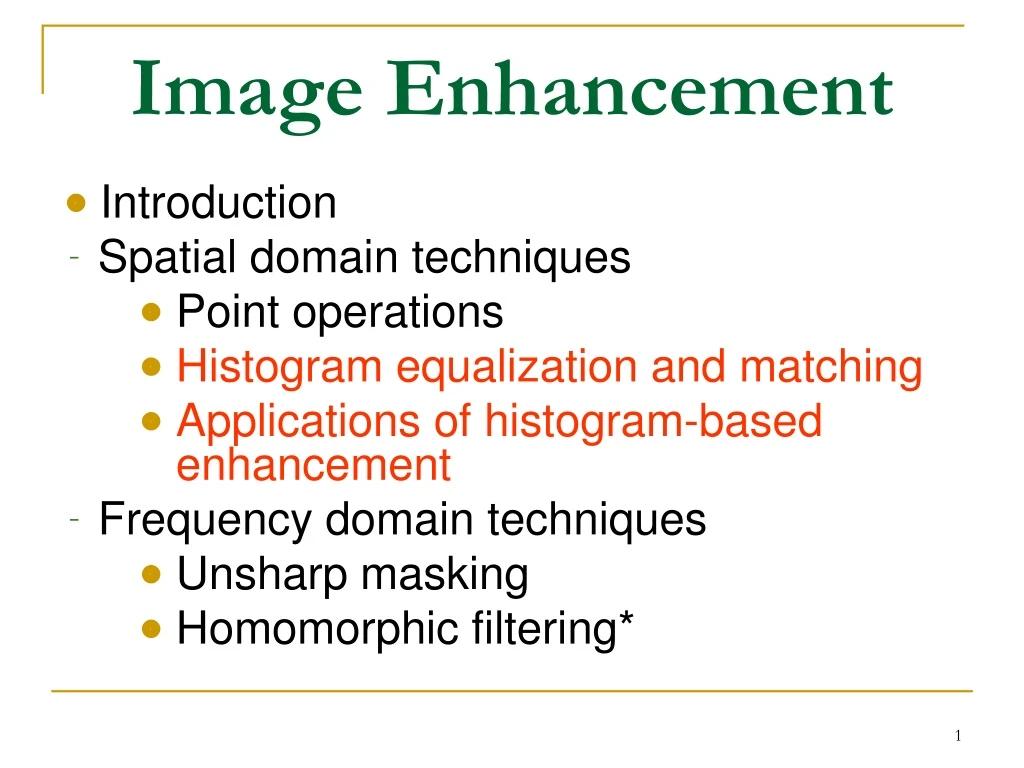
1. Image Enhancement • Introduction • Spatial domain techniques • Point operations • Histogram equalization and matching • Applications of histogram-based enhancement • Frequency domain techniques • Unsharp masking • Homomorphic filtering*

2. IMAGE ENHANCEMENT Point-wise operations Contrast enhancement; contrast stretching Grey scale clipping; image binarization (thresholding) Image inversion (negative) Grey scale slicing Bit extraction Contrast compression Image subtraction Histogram modeling: histogram equalization/ modification

3. Spatial operations Spatial low-pass filtering. Spatial high-pass and band-pass filtering Inverse contrast ratio mapping and statistical scaling Magnification and interpolation (image zooming) • Examples of image enhancement operations: • noise removal; • geometric distortion correction; • edge enhancement; • contrast enhancement; • image zooming; • image subtraction.

4. Recall: • There is no boundary of imagination in the virtual world • In addition to geometric transformation (warping) techniques, we can also photometrically transform images • Ad-hoc tools: point operations • Systematic tools: histogram-based methods • Applications: repair under-exposed or over-exposed photos, increase the contrast of iris images to facilitate recognition, enhance microarray images to facilitate segmentation.

5. Point Operations Overview Point operations are zero-memory operations where a given gray level x[0,L] is mapped to another gray level y[0,L] according to a transformation y L x L L=255: for grayscale images

6. m m n n U[M×N] V[M×N] Point-wise operation (grey scale transformation) f(∙) => v=f(u) u(m,n) v(m,n) = f(u(m,n)) A. Point-wise operations Def.: The new grey level (color) value in a spatial location (m,n) in the resulting image depends only on the grey level (color) in the same spatial location (m,n) in the original image => “point-wise” operation, or grey scale transformation (for grey scale images).

7. Lazy Man Operation y L x L No influence on visual quality at all

8. Digital Negative L x 0 L

9. Contrast Stretching yb ya x a b 0 L

10. Clipping x a b 0 L

11. Grey scale clipping; image thresholding • Grey scale clipping is a particular case of contrast enhancement, for m=p=0:

12. Range Compression x 0 L c=100

13. - Convolution mask AM SPATIAL OPERATIONS: most of them can be implemented by convolution

14. Histogram equalization and pseudo-coloring in biomedical images:

15. Summary of Point Operation • So far, we have discussed various forms of mapping function f(x) that leads to different enhancement results • MATLAB function >imadjust • The natural question is: How to select an appropriate f(x) for an arbitrary image? • One systematic solution is based on the histogram information of an image • Histogram equalization and specification

16. Histogram based Enhancement Histogram of an image represents the relative frequency of occurrence of various gray levels in the image MATLAB function >imhist(x)

17. Why Histogram? It is a baby in the cradle! Histogram information reveals that image is under-exposed

18. Another Example Over-exposed image

19. How to Adjust the Image? Histogram equalization Basic idea: find a map f(x) such that the histogram of the modified (equalized) image is flat (uniform). Key motivation: cumulative probability function (cdf) of a random variable approximates a uniform distribution Suppose h(t) is the histogram (pdf)

20. Histogram Equalization Uniform Quantization Note: y cumulative probability function L 1 x L 0

21. MATLAB Implementation function y=hist_eq(x) [M,N]=size(x); for i=1:256 h(i)=sum(sum(x= =i-1)); End y=x;s=sum(h); for i=1:256 I=find(x= =i-1); y(I)=sum(h(1:i))/s*255; end Calculate the histogram of the input image Perform histogram equalization

22. Image Example after before

23. Histogram Comparison after equalization before equalization

24. Adaptive Histogram Equalization

25. Histogram Specification/Matching Given a target image B, how to modify a given image A such that the histogram of the modified A can match that of target image B? histogram1 histogram2 S-1*T T S ?

26. Application (I): Digital Photography

27. Application (II): Iris Recognition after before

28. Application (III): Microarray Techniques after before

29. Application (IV)

30. Image Enhancement • Introduction • Spatial domain techniques • Point operations • Histogram equalization and matching • Applications of histogram-based enhancement • Frequency domain techniques • Unsharp masking • Homomorphic filtering*

31. Frequency-Domain Techniques (I): Unsharp Masking g(m,n) is a high-pass filtered version of x(m,n) • Example (Laplacian operator)

32. MATLAB Implementation % Implementation of Unsharp masking function y=unsharp_masking(x,lambda) % Laplacian operation h=[0 -1 0;-1 4 -1;0 -1 0]/4; dx=filter2(h,x); y=x+lambda*dx;

33. 1D Example xlp(n) x(n) g(n)=x(n)-xlp(n)

34. Frequency-Domain Techniques (II): Homomorphic filtering Basic idea: Illumination (low freq.) reflectance (high freq.) freq. domain enhancement

35. Summary of Nonlinear Image Enhancement • Understand how image degradation occurs first • Play detective: look at histogram distribution, noise statistics, frequency-domain coefficients… • Model image degradation mathematically and try inverse-engineering • Visual quality is often the simplest way of evaluating the effectiveness, but it will be more desirable to measure the performance at a system level • Iris recognition: ROC curve of overall system • Microarray: ground-truth of microarray image segmentation result provided by biologists

36. Spatial Image Enhancement Techniques: Image Averaging • A noisy image: • Averaging M different noisy images:

37. Image Averaging • As M increases, the variability of the pixel values at each location decreases. • This means that g(x,y) approaches f(x,y) as the number of noisy images used in the averaging process increases. • Registering of the images is necessary to avoid blurring in the output image.

38. Local Enhancement • When it is necessary to enhance details over smaller areas • To devise transformation functions based on the gray-level distribution in the neighborhood of every pixel

39. Local Enhancement • The procedure is: • Define a square (or rectangular) neighborhood and move the center of this area from pixel to pixel. • At each location, the histogram of the points in the neighborhood is computed and either a histogram equalization or histogram specification transformation function is obtained.

40. Local Enhancement • More procedure: • This function is finally used to map the grey level of the pixel centered in the neighborhood. • The center is then moved to an adjacent pixel location and the procedure is repeated.

41. Spatial Filtering • Use of spatial masks for image processing (spatial filters) • Linear and nonlinear filters • Low-pass filters eliminate or attenuate high frequency components in the frequency domain (sharp image details), and result in image blurring.

42. Spatial Filtering • High-pass filters attenuate or eliminate low-frequency components (resulting in sharpening edges and other sharp details). • Band-pass filters remove selected frequency regions between low and high frequencies (for image restoration, not enhancement).

43. Spatial Filtering a=(m-1)/2 and b=(n-1)/2, m x n (odd numbers) • For x=0,1,…,M-1 and y=0,1,…,N-1 • Also called convolution (primarily in the frequency domain)

44. Spatial Filtering • The basic approach is to sum products between the mask coefficients and the intensities of the pixels under the mask at a specific location in the image: (for a 3 x 3 filter)

45. Spatial Filtering • Non-linear filters also use pixel neighborhoods but do not explicitly use coefficients • e.g. noise reduction by median gray-level value computation in the neighborhood of the filter

46. Smoothing Filters • Used for blurring (removal of small details prior to large object extraction, bridging small gaps in lines) and noise reduction. • Low-pass (smoothing) spatial filtering • Neighborhood averaging - Results in image blurring

47. Image Enhancement in the Spatial Domain

48. Image Enhancement in the Spatial Domain

49. Smoothing Filters • Median filtering (nonlinear) • Used primarily for noise reduction (eliminates isolated spikes) • The gray level of each pixel is replaced by the median of the gray levels in the neighborhood of that pixel (instead of by the average as before).

50. Image Sharpening • Image sharpening deals with enhancing detail information in an image. • The detail information is typically contained in the high spatial frequency components of the image. • Therefore, most of the techniques contain some form of highpass filtering.