Download
1 / 13
130 likes | 136 Views
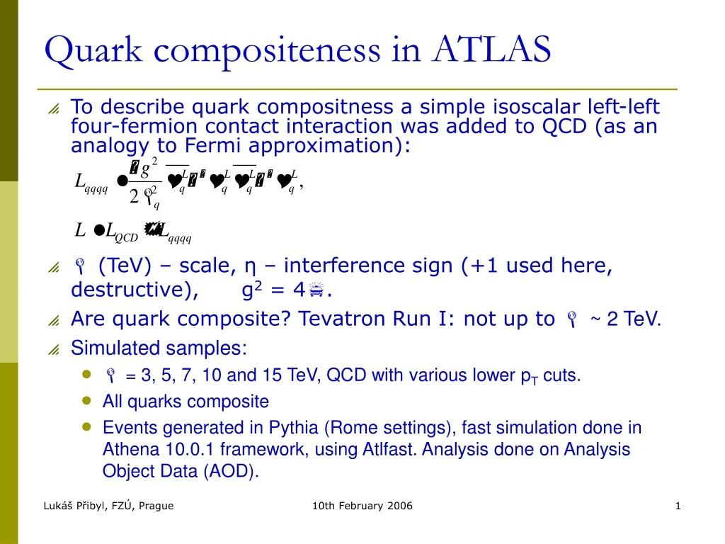
Quark c omposit e ness in ATLAS. To describe quark compositness a simple isoscalar left-left four-fermion contact interaction was added to QCD (as an analogy to Fermi approximation):. (TeV) – scale, η – interference sign (+1 used here, destructive) , g 2 = 4 .

E N D
Quark compositeness in ATLAS • To describe quark compositness a simple isoscalar left-left four-fermion contact interaction was added to QCD (as an analogy to Fermi approximation): • (TeV) – scale, η – interference sign (+1 used here, destructive), g2 = 4. • Are quark composite? Tevatron Run I: not up to ~ 2 TeV. • Simulated samples: • = 3, 5, 7, 10 and 15 TeV, QCD with various lower pT cuts. • All quarks composite • Events generated in Pythia (Rome settings), fast simulation done in Athena 10.0.1 framework, using Atlfast. Analysis done on Analysis Object Data (AOD). 10th February 2006
Quark compositness • What is investigated: • Inclusivejet production cross-section d/dpT.For high pTthe contact term above (CT) causes excess of events above standard QCD pT spectrum. pT spectrum is sensitive to PDF uncertainties and systematics (e.g. calorimeter nonlinearity). This effect can mask or fake compositness scenario. • Dijet angular distribution. Contact term causes excess of events with small pseudorapidity. Smaller dependance on systematics. 10 fb-1 5 TeV 7 TeV 10 TeV 15 TeV QCD 10th February 2006
Inclusivejet production cross-section • To characterize the excess of high-pT events one can use: 10 fb-1 5 TeV 7 TeV 10 TeV 15 TeV QCD • ET0:=1500 GeV. • =15 TeV is not obvious here. 10th February 2006
Inclusivejet production cross-section • What effect a calorimeter nonlinearity will make? • To parametrize nonlinearity of ATLAS hadronic calorimeter (simple method): • e/h - noncompensation, b – nonlinearity (smaller values achievable by e.g. weighting method) • c makes nonlin. and lin. spectra equal at 500 GeV. 10 fb-1 5 TeV 7 TeV 10 TeV 15 TeV b = 0.025, 1.5% @ 3TeV b = 0.11, 5.4% @ 3TeV 10th February 2006
Dijet angular distibution - Rχ • We need something less sensitive to calo nonlinearity and more unique to compositeness (inclusive jet c.s is similar to graviton)- dijet angular distribution. • Two leading jets with η1,η2. 20 fb-1 5 TeV 7 TeV 10 TeV 15 TeV QCD • To characterize this distribution: • χmax = 20 • χcut= 2.3 to 4 (to get the largest difference between and SM) 10th February 2006
R1 and R2 • Way to quantify difference between SM QCD and QCD+CT: 5 TeV 7 TeV 10 TeV 15 TeV • R2 gives significantly lower values, therefore not used further (might be different when systematics included). 10th February 2006
Selection of cuts – χcut pT > 1 TeV 5 TeV Dijet invariant mass cut: 20 fb-1 7 TeV 10 TeV 15 TeV mjj > 3 TeV QCD No mjj upper cut used (uneffective). Many pT (1 TeV and higher) and mjj cuts tried. For each pT and mjj cut a χcut was chosen to give max R1. mjj > 6 TeV 10th February 2006
Selection of cuts - mjj • Best χcut’s already used • Best mjj cuts found for given and pT cut (here 1 TeV). 5 TeV 7 TeV 10 TeV 15 TeV 10th February 2006
R1 vs. pT • Even at 100 pb-1 R1(7 TeV) > 3. • To spot 5 TeV even smaller int. luminosity is enough (no systematics). 5 TeV 7 TeV 10 TeV 15 TeV 10th February 2006
R1 vs. pT 5 TeV 7 TeV 10 TeV 15 TeV • The lower pT cut the higher R1 – simulation with smaller CKIN(3) is useful. The lower pT cut the larger number of events! • The lowest limit for pT comes from trigger, but hopefully a plateau is reached at higher pT’s, especially for high , where high int. luminosity is necessary. If not – technically difficult. 10th February 2006
R1 vs. pT 5 TeV 7 TeV 10 TeV 15 TeV • Values of integral luminosity to reach R1 = 3 for various compositeness scales: No systematic errors included. 10th February 2006
R1, pT > 550 GeV 3 TeV 5 TeV 7 TeV 10 TeV • CKIN(3) = 350. • Compare with ATLAS HLT triggers: • j400, 2j350, 3j165, 4j110 • Available data: 1 inv.fb, =3,5,7,10 TeV. • Required lumi. decreased 2-3x. • No systematics included. 10th February 2006
Conclusions • Now it seems, that to spot (or rule out) small compositness scales(5 TeV), a few days of datataking should be enough(15 pb-1). • Looking at data with lower pT cut makes this time even shorter. • When systematic errors (PDF uncertainties, jet algorithms,...) are included, this time will be prolonged (to be studied). • A model with negative (constructive) interference should be discovered (or ruled out) even sooner. • Discovery limits are still not definitive. 10th February 2006