Download
1 / 31
310 likes | 431 Views
MSc in High Performance Computing Computational Chemistry Module Parallel Molecular Dynamics (ii). Bill Smith CCLRC Daresbury Laboratory w.smith@daresbury.ac.uk. Basic MD Parallelization Strategies. Recap: Last Lecture Computing Ensemble Hierarchical Control Replicated Data

E N D
MSc in High Performance ComputingComputational Chemistry ModuleParallel Molecular Dynamics (ii) Bill Smith CCLRC Daresbury Laboratory w.smith@daresbury.ac.uk
Basic MD Parallelization Strategies Recap: • Last Lecture • Computing Ensemble • Hierarchical Control • Replicated Data • This Lecture • Systolic Loops • Domain Decomposition
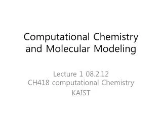
P 2 1 P-1 P+1 2P P+2 2P-1 Proc (P-1) Proc 0 Proc 1 Proc (P- 2) Systolic Loops: SLS-G Algorithm • Systolic Loop algorithms • Compute the interactions between (and within) `data packets’ • Data packets are then transferred between nodes to permit calculation of all possible pair interactions
Systolic Loop (SLS-G) Algorithm • Systolic Loop Single-Group • Features: • P processing nodes, N molecules • 2P groups (`packets’) of n molecules (N=2Pn) • For each time step: • (a) calculate intra-group forces • (b) calculate inter-group forces • (c) move data packets one `pulse’ • (d) repeat (b)-(c) 2P-1 times • (e) integrate equations of motion
Systolic Loop Performance Analysis (i) Processing Time: Communications Time: with
Systolic Loop Performance Analysis (ii) Fundamental Ratio: Large N (N>>P): Small N (N~2P):
Systolic Loop Algorithms • Advantages • Good load balancing • Portable between parallel machines • Good type 1 scaling with system size and processor count • Memory requirement fully distributed • Asynchronous communications • Disadvantages • Complicated communications strategy • Complicated force fields difficult
B A C D Domain Decomposition (Parallel - 2D)
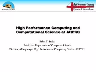
(b) (a) Domain Decomposition (Parallel - 3D)
Domain Decomposition MD • Features: • Short range potential cut off (rcut << Lcell) • Spatial decomposition of atoms into domains • Map domains onto processors • Use link cells in each domain • Pass border link cells to adjacent processors • Calculate forces, solve equations of motion • Re-allocate atoms leaving domains
Domain Decomposition Performance Analysis (i) • Processing Time: • Communications Time: • with • and is the number of link cells per node. NB: O(N) Algorithm
Fundamental Ratio: Large N Case 1: (N>>P and fixed): Large N Case 2: (N>>P and i.e. fixed): Small N: (N=P and ): Domain Decomposition Performance Analysis (ii)
Domain Decomposition MD • Advantages: • Predominantly Local Communications • Good load balancing (if system is isotropic!) • Good type 1 scaling • Ideal for huge systems (105 ~ 105 atoms) • Simple communication structure • Fully distributed memory requirement • Dynamic load balancing possible • Disadvantages • Problems with mapping/portability • Sub-optimal type 2 scaling • Requires short potential cut off • Complex force fields tricky
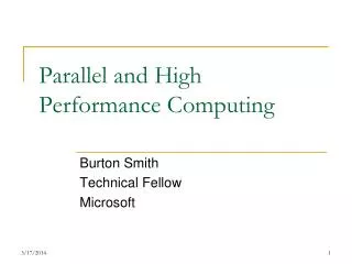
P0Local atomic indices P1Local atomic indices P2Local atomic indices Force field definition Global atomic indices Difficult! Processor Domains Domain Decomposition: Intramolecular Forces
The crucial part of the SPME method is the conversion of the Reciprocal Space component of the Ewald sum into a form suitable for Fast Fourier Transforms (FFT). Thus: becomes: whereG and Q are 3D grid arrays (see later) Coulombic Forces: Smoothed Particle-Mesh Ewald Ref: Essmann et al., J. Chem. Phys. (1995) 103 8577
SPME: Spline Scheme Central idea - share discrete charges on 3D grid: Cardinal B-Splines Mn(u) - in 1D: Recursion relation
SPME: Building the Arrays Is the charge array and QT(k1,k2,k3) its discrete Fourier transform. GT (k1,k2,k3) is the discrete Fourier Transform of the function: with
SPME Parallelisation • Handle real space terms using short range force methods • Reciprocal space terms options: • Fully replicated Q array construction and FFT (R. Data) • Atomic partition of Q array, replicated FFT (R. Data) • Easily done, acceptable for few processors • Limits imposed by RAM, global sum required • Domain decomposition of Q array, distributed FFT • Required for large Q array and many processors • Atoms `shared’ between domains - potentially awkward • Requires distributed FFT - implies comms dependence
SPME: Parallel Approaches • SPME is generally faster then conventional Ewald sum in most applications. Algorithm scales as O(NlogN) • In Replicated Data: build the FFT array in pieces on each processor and make whole by a global sum for the FFT operation. • In Domain Decomposition: build the FFT array in pieces on each processor and keep that way for the distributed FFT operation (The FFT `hides’ all the implicit communications) • Characteristics of FFTs • Fast (!) - O(M log M) operations where M is the number of points in the grid • Global operations - to perform a FFT you need all the points • This makes it difficult to write an efficient, good scaling FFT.
Traditional Parallel FFTs • Strategy • Distribute the data by planes • Each processor has a complete set of points in the x and y directions so can do those Fourier transforms • Redistribute data so that a processor holds all the points in z • Do the z transforms • Characteristics • Allows efficient implementation of the serial FFTs ( use a library routine ) • In practice for large enough 3D FFTs can scale reasonably • However the distribution does not usually map onto domain decomposition of simulation - implies large amounts of data redistribution
Daresbury Advanced 3-D FFT (DAFT) • Takes data distributed as MD domain decomposition. • So do a distributed data FFT in the x direction • Then the y • And finally the z • Disadvantage is that can not use the library routine for the 1D FFT ( not quite true – can do sub-FFTs on each domain ) • Scales quite well - e.g. on 512 procs, an 8x8x8 proc grid, a 1D FFT need only scale to 8 procs • Totally avoids data redistribution costs • Communication is by rows/columns • In practice DAFT wins ( on the machines we have compared ) and also the coding is simpler !
Domain Decomposition: Load Balancing Issues • Domain decomposition according to spatial domains sometimes presents severe load balancing problems • Material can be inhomogeneous • Some parts may require different amounts of computations • E.g. enzyme in a large bath of water • Strategies can include • Dynamic load balancing: re-distribution (migration) of atoms from one processor to another • Need to carry around associated data on bonds, angles, constraints….. • Redistribution of parts of the force calculation • E.g. NAMD
Domain Decomposition: Dynamic Load Balancing Can be applied in 3D (but not easily!) Boillat, Bruge, Kropf, J. Comput Phys., 96 1 (1991)
NAMD: Dynamic Load Balancing • NAMD exploits MD as a tool to understand the structure and function of biomolecules • proteins, DNA, membranes • NAMD is a production quality MD program • Active use by biophysicists (science publications) • 50,000+ lines of C++ code • 1000+ registered users • Features and “accessories” such as • VMD: visualization and analysis • BioCoRE: collaboratory • Steered and Interactive Molecular Dynamics • Load balancing ref: • L.V. Kale, M. Bhandarkar and R. Brunner, Lecture Notes in Computer Science 1998, 1457, 251-261.
NAMD : Initial Static Balancing • Allocate patches (link cells) to processors so that • Each processor has same number of atoms (approx.) • Neighbouring patches share same processor if possible • Weighing the workload on each processor • Calculate forces internal to each patch (weight ~ np2/2) • Calculate forces between patches (i.e. one compute object) on the same processor (weight ~ w*n1*n2). Factor w depends on connection (face-face > edge-edge > corner-corner) • If two patches on different processors – send proxy patch to lesser loaded processor. • Dynamic load balancing used during simulation run.
NAMD : Dynamic Load Balancing (i) • Balance maintained by a Distributed Load Balance Coordinator which monitors on each processor: • Background load (non migratable work) • Idle time • Migratable compute objects and their associated compute load • The patches that compute objects depend upon • The home processor of each patch • The proxy patches required by each processor • The monitored data is used to determine load balancing
NAMD : Dynamic Load Balancing (ii) • Greedy load balancing strategy: • Sort migratable compute objects in order of heaviest load • Sort processors in order of `hungriest’ • Share out compute objects so hungriest ranked processor gets largest compute object available • BUT: this does not take into account communication cost • Modification: • Identify least loaded processors with: • Both patches or proxies to complete a compute object (no comms) • One patch necessary for a compute object (moderate comms) • No patches for a compute object (high comms) • Allocate compute object to processor giving best compromise in cost (compute plus communication).