Download
1 / 20
200 likes | 223 Views
Explore the relationship between parent and child heights using Galton’s data, predict child height based on parent height in this regression analysis. Learn about least squares regression method, intercepts, coefficients interpretation, and model assumptions.

E N D
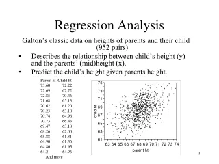
Regression Analysis Galton’s classic data on heights of parents and their child (952 pairs) • Describes the relationship between child’s height (y) and the parents’ (mid)height (x). • Predict the child’s height given parents height. Parent ht Child ht 73.60 72.22 72.69 67.72 72.85 70.46 71.68 65.13 70.62 61.20 70.23 63.10 70.74 64.96 70.73 66.43 69.47 63.10 68.26 62.00 65.88 61.31 64.90 61.36 64.80 61.95 64.21 64.96 And more
Uses of Regression Analysis • Description: Describe the relationship between a dependent variable y (child’s height) and explanatory variables x (parents’ height). • Prediction: Predict dependent variable y based on explanatory variables x.
Model for Simple Regression Model • Consider a population of units on which the variables (y,x) are recorded. • Let denote the conditional mean of y given x. • The goal of regression analysis is to estimate . • Simple linear regression model:
Simple Linear Regression Model • Model (more details later) y = dependent variable x = independent variable b0 = y-intercept b1 = slope of the line e = error (normally distributed) b0 and b1 are unknown populationparameters, therefore are estimated from the data. Rise b1 = Rise/Run Run b0 x
Interpreting the Coefficients • The slope is the change in the mean of y that is associated with a one unit change in x e.g.,for each extra inch for parents, the average heights of the child increases by 0.6 inch. • The intercept is the estimated mean of y for x=0. However, this interpretation should only be used when the data contains observations with x near 0. Otherwise it is an extrapolation of the model which can be unreliable (Section 3.7.2). child ht = 26.46 + 0.6 parent ht
Estimating the Coefficients • The estimates are determined from • observations: (x1,y1),…,(xn,yn). • by calculating sample statistics. • Correspond to a straight line that cuts into the data. Question: What should be considered a good line? y w w w w w w w w w w w w w w w x
Least Squares Regression Line • What is a good estimate of the line? • A good estimated line should predict y well based on x. • Least absolute value regression line: Line that minimizes the absolute values of the prediction errors in the sample. Good criterion but hard to compute. • Least squares regression line: Line that minimizes the squared prediction errors in the sample. Good criterion and easy to compute.
Sum of squared differences = (2 -2.5)2 + (4 - 2.5)2 + (1.5 - 2.5)2 + (3.2 - 2.5)2 = 3.99 1 1 The Least Squares (Regression) Line Sum of squared differences = (2 - 1)2 + (4 - 2)2 + (1.5 - 3)2 + (3.2 - 4)2 = 6.89 Let us compare two lines (2,4) 4 The second line is horizontal w (4,3.2) w 3 2.5 2 w (1,2) (3,1.5) w The smaller the sum of squared differences the better the fit of the line to the data. 2 3 4
The Estimated Coefficients To calculate the estimates of the coefficients of the line that minimizes the sum of the squared differences between the data points and the line, use the formulas: The regression equation that estimates the equation of the simple linear regression model is:
Example Heights (cont.) • In R • sl<-lm(Child~Parent) • summary(sl) • plot(Parent,Child) • points(Parent,fitted.values(sl),type="l",col="red")
Call: lm(formula = Child ~ Parent) Residuals: Min 1Q Median 3Q Max -8.44126 -1.55205 0.06787 1.61437 5.83156 Coefficients: Estimate Std. Error t value Pr(>|t|) (Intercept) 26.45556 2.91962 9.061 <2e-16 *** Parent 0.61152 0.04275 14.303 <2e-16 *** --- Signif. codes: 0 ‘***’ 0.001 ‘**’ 0.01 ‘*’ 0.05 ‘.’ 0.1 ‘ ’ 1 Residual standard error: 2.357 on 950 degrees of freedom Multiple R-squared: 0.1772, Adjusted R-squared: 0.1763 F-statistic: 204.6 on 1 and 950 DF, p-value: < 2.2e-16
Ordinary Linear Model Assumptions • Properties of errors under ideal model: • for all x. • for all xi • The distribution of is normal. • are independent. • and • Equivalent definition: For each , has a normal distribution with mean and variance . Also, are independent.
Typical Regression Analysis • Observe pairs of data (x1,y1),…,(xn,yn) that are a sample from population of interest. • Plot the data. • Assume simple linear regression model assumptions hold. • Estimate the true regression line by the least squares line • Check whether the assumptions of the ideal model are reasonable (Chapter 6, and next lecture) • Make inferences concerning coefficients and make predictions ( )


