Download
1 / 64
640 likes | 783 Views
Micro Scale Meteorology Grænselags Meteorologi. Søren E.Larsen soeren.larsen@risoe.dk Vindenergi Afdelingen Risø. Praktikaliteter: Ca 45 forelæsningeruger. Hvordan og hvornår aftales ved første forelæsning. Lige nu har vi mandag og onsdag. Mundtlig eksamen

E N D
Micro Scale MeteorologyGrænselags Meteorologi Søren E.Larsen soeren.larsen@risoe.dk Vindenergi Afdelingen Risø
Praktikaliteter: • Ca 45 forelæsningeruger. Hvordan og hvornår aftales ved første forelæsning. Lige nu har vi mandag og onsdag. • Mundtlig eksamen • Baseret på uddelte noter, anbefalede bøger • 7.5ECTS
Microscale Meteorology Søren E. Larsen Department of Wind Energy Risø National Laboratory, Denmark Content 1 Introduction 2 Concepts, Statistical tools and Scales of Motio 3 Basic Equations 4 Equations and closures 5 Simple Boundary Layers, Ekman Spiral 6 Surface Layer, Monin-Obuchov and other scaling
7 Near Surface Viscuous Layers, z0, z0T ,Interfacial Exchange. 8 Scaling Regimes in the Atmospheric Boundary Layer 9 Heterogeneous Atmospheric Boundary Layer 10 Atmospheric Dispersion 12 Wind Resources 13 Climatology 14 Measurement techniques and principles 15 Literature
Literature: Notes are on: http://www.risoe.dk/vea/thesis/LecturesCourses.htm.
1. lectures The first lectures focus on illustrating the behaviour of the atmospheric boundary layer by use of informative figures, as found in the literature. We start with the structure of the whole atmosphere. Here the boundary layer is at the far bottom being less or about than one kilometer in depth.
Strukture of the atmosphere • Ionosphere • Mesosphere • Stratosphere • Troposphere • Atm. boundary layer • Surface layer
CO2, CH4, H2O Greenhouse gases absorb long wave radiation O3 Absorbs shortwave radiation
Clouds and aerosols Aerosols are airborne particles typically organised in size spectra. Clouds consists of water droplets, condensed from the atmospheric water vapour field. The water droplets in clouds are condenced around an aerosol particle, denoted a cloud condensation nuclei. Clouds and aerosols influences the radiation budget, mostly by reflection.
Aerosols • Aerosols are produced from the surfaces (dust and water spray and transported upwards). • Aerosols are as well produced by nucleation from gases in the atmosphere. • There are problems by closing the Earth’s aerosol budget. • Aerosols varies in size, nanometers-mm, and in composition.
Results: • Particle size spectra conditionally sampled by wind direction and speed indicate flow from the land exhibits higher sub-micron particle numbers while flow from the marine fetch exhibits higher concentrations for D = 1 – 5 m. Particle size spectra conditionally sampled by wind speed and direction.
Results: • Particle composition data from the MOUDIs during the August 2000 experiment indicate significant coarse mode NO3-, while NH4+ is largely confined to the accumulation mode. Measured size resolved particle composition (from the MOUDIs) during the 2000 field experiment at Ringhals.
Incoming solar radiation 342 W m-2 Outgoing longwave radiation 235 W m-2 342 107 Emitted by Atmosphere 195 W m-2 Reflected solar radiation 107 W m-2 195 Atmospheric Window 40 40 Absorbed by atmosphere 67 W m-2 Reflected by clouds, Aerosols and atmosphere 77 W m-2 67 Absorbed by Clouds and GHG 350 W m-2 77 Latent heat 78 390 24 324 78 Reflected by surface 30 W m-2 168 back Radiation 30 Absorbed by surface 168 W m-2 Thermals 24 Surface Radiation 390 Evapo Transpiration 78
Scales of motion • Global scale • Global circulation • Synoptic scale motion • meso-scale motion • micro-scale motion • boundary layers
Den geostrofiske vind • Corriolis kraften • trykgradienter
Thermosphere Mesopause 80 km Coldest temperature Mesosphere Stratopause 50 km O + O2 +M → O3 Stratosphere Vitually no mixing very slow removal Tropopause 10 km Troposphere PBL 0 C -60 C 60 C
Variationer i vinden Zooming in on a 100 days wind record: The zooming to the next figure is indicated by the grey area. Each graph consists of 1200 data, averaged over 1/1200 of the period
The atmospheric boundary layer. The atmospheric boundary layer is the atmospheric layer close to the ground, where the surface friction brakes the air speed to zero. Hence it is the layer where the wind speed at the top equals the wind speed in the free atmosphere. Close to the surface the wind speed is reduced to the speed of the surface ~ 0 meter/second. As the wind is a vector and the stress is a vector or a tensor the wind changes through the boundary layer both in speed and direction, see following figure. The lowest roughly 10% of the boundary layer is called the surface layer. Here the turning of the wind is negligible. The next slides show different perspectives of the variation of the wind speed and direction through the boundary layer, the so called Ekman Spiral.
Geostrophic drag law • In the free atmosphere: • Balance between pressure force and • Coriolis force
Geostrophic drag law At the surface: Add frictional force
The Eksman Spiral seen from above. From z =0, the end of the velocity vector will trace the curve until the the top of the boundary layer, where wind becomes Geostrophic, G, with components Ug and Vg.
Diurnal variations of the atmospheric boundary layer The atmospheric boundary layer varies during the day in response to the radiational heating (during day) and cooling of the ground (during night). During a sunny day the boundary layer flow is said to be thermally unstable, because the heating at the ground makes the air lighter than aloft. During nighttime the air is coldest near the ground at the atmosphere is said to be stable.
Diurnal growths of the ABL Diurnal variation
Typisk ”Klar himmel” grænselag Overfladegrænselaget ca. 1/10 af inversionshøjden
More about the boundary layer, its stability and the flow structures for different situations: Eddies
Atmosfærisk stabilitetUstabilt (konvektivt) • Ustabilt : Lave vindhastigheder med solskin. Varme bobler af luft stiger fra overfladen
Atmosfærisk stabilitetStabilt • Stabile forhold : lave vindhastigheder og en kold overflade e.ks stille nat uden skyer eller kun meget lidt skydække • Kold luft akkumuleres ved overfladen og løber ned af skråninger mm.
Typical boundary layer profiles of • wind speed,U, temperature, T, • and water vapour mixing ratio, q: • Daytime unstable conditions. Part of the profiles are well mixed,i.e. no height variation. • Night time stable conditions. Stronger height variation of profiles. • Thermally neutral conditions. The profiles are logarithmic in a height interval.
Importance of the boundary stability and flow conditions for dispersion of air pollution.
All atmospheric variables vary on a very broad range of spatial and temporal scales. Timescales from Megayears to milliseconds. Spatial scales from Megameters to millimeters
Variationer i vinden Zooming in on a 100 days wind record: The zooming to the next figure is indicated by the grey area. Each graph consists of 1200 data, averaged over 1/1200 of the period