Download
1 / 41
410 likes | 490 Views
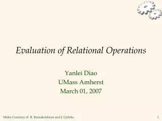
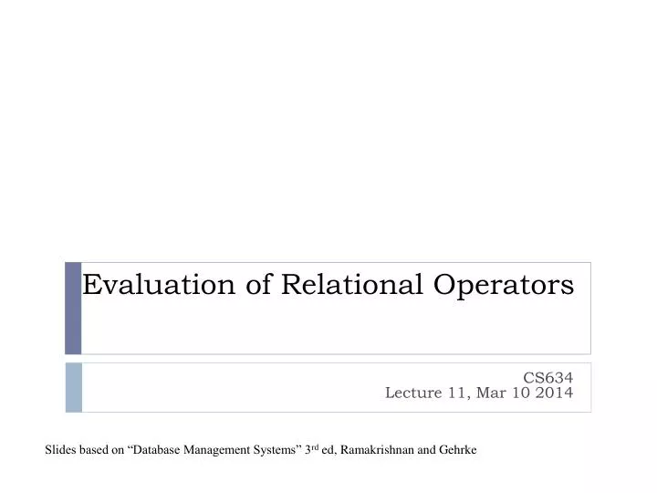
Evaluation of Relational Operators. CS634 Lecture 11, Mar 10 2014. Slides based on “Database Management Systems” 3 rd ed , Ramakrishnan and Gehrke. Architecture of a DBMS. User. SQL Query. Query Compiler. Query Plan (optimized). Execution Engine. Index and Record requests.

E N D
Evaluation of Relational Operators CS634Lecture 11, Mar 10 2014 • Slides based on “Database Management Systems” 3rded, Ramakrishnan and Gehrke
Architecture of a DBMS • User • SQL Query Query Compiler • Query Plan (optimized) Execution Engine • Index and Record requests Index/File/Record Manager • Page Commands Buffer Manager • Read/Write pages Disk Space Manager • Disk I/O Data • A first course in database systems, 3rded, Ullman and Widom
Relational Algebra • Relational operators: • Selection • Projection • Join Combines several relations using conditions • Set-differenceUnionIntersection • Aggregation and Grouping
Example Schema • Similar to old schema; rnameadded • Reserves: • 40 bytes long tuple, 100K records, 100 tuples per page, 1000 pages • Sailors: • 50 bytes long tuple, 40K tuples, 80 tuples per page, 500 pages Sailors (sid: integer, sname: string, rating: integer, age: real) Reserves (sid: integer, bid: integer, day: dates, rname: string)
Selections with Simple Condition • Case 1: No index, Unsorted data • Do scan • Case 2: No Index, Sorted Data • Perform binary search on file (exact match or ranges) • O(log M), M = number of pages in file • Case 3: Index Available • Is the index B+-Tree or Hash? • Is it clustered or not?
Using an Index for Selections • Cost depends on • Number of qualifying tuples • Clustering • Cost has two components: • Finding qualifying data entries (typically small) • Retrieving records (could be large w/o clustering) • Consider Reserves, assume 10% of tuples satisfy condition • Result has 10K tuples, 100 pages • With clustered index, cost is little more than 100 I/Os • If unclustered, up to 10000 I/Os!
For Unclustered Indexes • Important refinement: 1. Find qualifying data entries 2. Sort the rid’s of the data records to be retrieved 3. Fetch rids in order • Ensures that each data page is looked at just once • although number of I/Os still higher than with clustering
General Conditions Selections • Condition may be composite • In conjunctive form: easier to deal with • At least one disjunction: less favorable case • Disjunctive form • Only one of the conditions, if met, qualifies tuple • Even if some disjunct is optimized, the other(s) may require scan • In general, this case dealt with using set union • Most DBMS optimizers focus on conjunctive forms
Evaluating Conjunctive Forms (1/2) • Find the most selective access path, retrieve tuples using it, and apply any remaining terms that don’t match the index • Most selective access path: An index or file scan that we estimate will require the fewest page I/Os • Example: day<8/9/94 AND bid=5 AND sid=3 • B+ tree index on daycan be used; then, bid=5 and sid=3 must be checked for each retrieved tuple • Similarly, a hash index on <bid, sid> could be used; day<8/9/94 must then be checked.
Evaluating Conjunctive Forms (2/2) • Intersect rid’s • If we have two or more matching indexes that use Alternatives (2) or (3) for data entries: • Get sets of rids of data records using each matching index • Then intersectthese sets of rids (we’ll discuss intersection soon!) • Retrieve the records and apply any remaining terms • Example: day<8/9/94 AND bid=5 AND sid=3 • B+ tree index on day and an index on sid, both using Alternative (2) • Retrieve rids satisfying day<8/9/94using the B+ tree, rids satisfying sid=3 using the hash, intersect, retrieve records and check bid=5
Intersecting RIDs via Index JOIN • Example: day<8/9/94 AND bid=5 AND sid=3 • B+ tree index on day and an index on sid, both using Alternative (2) • Retrieve rids satisfying day<8/9/94using the B+ tree, rids satisfying sid=3 using the hash, intersect, retrieve records and check bid=5 • Another way to achieve this: Join the two indexes • As tables, indexes are I1 = (rid, day) and I2 = (rid, sid) • Join them: I1 where day<8/9/94 JOIN I2 where sid = 3 • Obtain (rid, day, sid) satisfying the two conditions and providing rids
Projection with Sorting • Modify Pass 0 of external sort to eliminate unwanted fields • Produce runs of about 2B pages are produced • Tuples in runs are smaller than input tuples • Size ratio depends on number and size of fields that are dropped • Modify merging passes to eliminate duplicates • Thus, number of result tuples smaller than input • Difference depends on number of duplicates • Cost • In Pass 0, read original relation (size M), write out same number of smaller tuples • In merging passes, fewer tuples written out in each pass. Using Reserves example, 1000 input pages reduced to 250 in Pass 0 if size ratio is 0.25
Projection with Hashing • Partitioning phase: • Read R using one input buffer. For each tuple, discard unwanted fields, apply hash function h1 to choose one of B-1output buffers • Each output buffer is feeding a run on disk • Result is B-1 partitions (of tuples with no unwanted fields), tuples from different partitions guaranteed to be distinct • See next slide for diagram • Duplicate elimination phase: process runs from partitioning phase. Each run forms a partition of the data
Original Relation Partitions OUTPUT 1 1 2 INPUT 2 hash function h . . . B-1 B-1 B main memory buffers Disk Disk Hash Projection: Partitioning Phase • Partition R using hash function h • Duplicates will hash to the same partition
Projection with Hashing • Partitioning phase: ends up with partitions of data, each held in a run on disk • Duplicate elimination phase: • For each partition, read it and build an in-memory hash table, using hash h2on all fields, while discarding duplicates • If partition does not fit in memory, can apply hash-based projection algorithm recursively to this partition • Cost • Read R, write out each tuple, but fewer fields, size T <= M. Result read in next phase. Total i/o cost: M + 2T<= 3M, similar to sort if it can be done in 2 passes.
Partitions of R Projection Result Hash table for partition Ri (k < B pages) hash fn h2 h2 Output buffer Input buffer for R B main memory buffers Disk Disk Hash Projection: Second Phase Read in a partition of R, hash it using h2 (<> h!) Discard duplicates as go along. When partition is all read in, scan the hash table and write it out as part of the projection result or
Discussion of Projection • Sort-based approach is the standard • better handling of skew and result is sorted. • Hashing is more parallelizable • If index on relation contains all wanted attributes in its search key, do index-onlyscan • Apply projection techniques to data entries (much smaller!) • If an ordered (i.e., tree) index contains all wanted attributes as prefixof search key, can do even better: • Retrieve data entries in order (index-only scan) • Discard unwanted fields, compare adjacent tuples to check for duplicates
Equality Joins With One Join Column • Most frequently occurring in practice • We will consider more complex join conditions later • Cost metric: number of I/Os • Ignore output costs SELECT * FROM Reserves R1, Sailors S1 WHERE R1.sid=S1.sid
Simple Nested Loops Join • For each tuple in the outer relation R, we scan the entire inner relation S. • Cost: M + pR * M * N = 1000 + 100*1000*500 I/Os • Page-oriented Nested Loops join: • For each page of R, get each page of S, and write out matching pairs • Cost: M + M*N = 1000 + 1000*500 • If smaller relation (S) is outer, cost = 500 + 500*1000 foreach tuple r in R do foreach tuple s in S do if ri == sj then add <r, s> to result
. . . Block Nested Loops Join • one page input buffer for scanning the inner S • one page as the output buffer • remaining pages to hold ``block’’ of outer R • For each matching tuple r in R-block, s in S-page, add <r, s> to result. Then read next R-block, scan S, etc. R & S Join Result Block of R (B-2 pages) . . . . . . Output buffer Input buffer for S
Examples of Block Nested Loops • Cost: Scan of outer + #outer blocks * scan of inner • #outer blocks = • With Reserves (R) as outer, and 100 pages per block: • Cost of scanning R is 1000 I/Os; a total of 10 blocks. • Per block of R, we scan Sailors (S); 10*500 I/Os. • Total 1000 + 10*500 = 6000 i/os. • With 100-page block of Sailors as outer: • Cost of scanning S is 500 I/Os; a total of 5 blocks. • Per block of S, we scan Reserves; 5*1000 I/Os. • Total 500 + 5*1000 = 5500 i/os. Same ballpark as above. • Compare these to page-oriented NLJ: 500,000 i/o or worse!
Executing Joins: Index Nested Loops • Cost = M + (M*pR) * (cost of finding matching S tuples) • M = number of pages of R, pR= number of R tuples per page • If relation has index on join attribute, make it inner relation • For each outer tuple, cost of probing inner index is 1.2for hash index, 2-4 for B+, plus cost to retrieve matching S tuples • Clustered index typically single I/O • Unclustered index 1 I/O per matching S tuple foreach tuple r in R do foreachtuple s in S where ri == sjdo add <r, s> to result
Example of Index Nested Loops (1/2) Case 1: Hash-index (Alternative2) on sid of Sailors • Choose Sailors as inner relation • Scan Reserves: 100K tuples, 1000 page I/Os • For each Reserves tuple • 1.2 I/Os to get data entry in index • 1I/O to get (the exactly one) matching Sailors tuple (primary key) • Total: 221,000 I/Os
Example of Index Nested Loops (2/2) Case 2: Hash-index (Alternative 2) on sid of Reserves • Choose Reserves as inner • Scan Sailors: 40K tuples, 500 page I/Os • For each Sailors tuple • 1.2I/Os to find index page with data entries • Assuming uniform distribution, 2.5 matching records per sailor • Cost of retrieving records is single I/O (clustered index) or 2.5 I/Os(unclustered index) • Total: 88,500 I/Os(clustered) or 148,500 I/Os(unclustered)
Sort-Merge Join • Sort R and S on the join column • Then scan them to do a merge on join column: • Advance scan of R until current R-tuple >= current S tuple • Then, advance scan of S until current S-tuple >= current R tuple • Repeat until current R tuple = current S tuple • At this point, all R tuples with same value in Ri (current R group) and all S tuples with same value in Sj (current S group) match • Output <r, s> for all pairs of such tuples • Resume scanning R and S
Sort-Merge Join Cost • R is scanned once • Each S group is scanned once per matching R tuple • Multiple scans per group needed only if S records with same join attribute value span multiple pages • Multiple scans of an S group are likely to find needed pages in buffer • Cost: (assume B buffers) • Sort(R) + Sort(S) + merge • 2M (1+log B-1(M/B)) + 2N (1+logB-1 (N/B)) + (M+N) • The cost of scanning, M+N, could be M*N worst case (very unlikely!) • In many cases, the join attribute is primary key in one of the tables, which means no duplicates in one merge stream.
2-Pass Sort-Merge Join • With enough buffers, sort can be done in 2 passes • First pass generates N/B sorted runs of B pages each • If one page from each run + output buffer fits in memory, then merge can be done in one pass; denote larger relation by L • 2L/B + 1 <= B, holds if (approx) B > • One optimization of sort allows runs of 2B on average • First pass generates N/2B sorted runs of 2B pages each • Condition above for 2-pass sort becomes B > • (But we’re not officially covering this optimization) • Merge can be combined with filtering of matching tuples • The cost of sort-merge join becomes 3(M+N)
Original Relations Partitions OUTPUT 1 1 2 INPUT 2 hash function h . . . B-1 B-1 B main memory buffers Disk Disk Hash-Join: Partitioning Phase • Partition both relations using hash function h • R tuples in partition i will only match S tuples in partition I • This is the similar to the partitioning phase of Projection by Hashing
Partitions of R & S Join Result Hash table for partition Ri (k < B-1 pages) hash fn h2 h2 Output buffer Input buffer for Si B main memory buffers Disk Disk Hash-Join: Probing Phase Read in a partition of R, hash it using h2 (<> h!) Scan matching partition of S, search for matches.
Hash-Join Properties • #partitions k <= B-1 because one buffer is needed for scanning input • Assuming uniformly sized partitions, and maximizing k: • k= B-1, and M/(B-1) <= B-2, i.e., B > • M is smaller of the two relations! • If we build an in-memory hash table to speed up the matching of tuples, slightly more memory is needed • If the hash function does not partition uniformly, one or more R partitions may not fit in memory • Can apply hash-join technique recursively to do the join of this R-partition with corresponding S-partition.
Cost of Hash-Join • In partitioning phase, read+write both R and S: 2(M+N) • In matching phase, read both R and S: M+N • With sizes of 1000 and 500 pages, total is 4500 I/Os
Hash-Join vs Sort-Merge Join • Given sufficient amount of memory both have a cost of 3(M+N)I/Os • Hash Join superior on this count if relation sizes differ greatly • Hash Join shown to be highly parallelizable • Sort-Merge less sensitive to data skew, and result is sorted
General Join Conditions (1/2) • Equalities over several attributes • e.g., R.sid=S.sidANDR.rname=S.sname • For Index Nested Loop, build index on<sid, sname> (if S is inner); or use existing indexes on sidor sname • For Sort-Merge and Hash Join, sort/partition on combination of the two join columns
General Join Conditions (2/2) • Inequality conditions • e.g., R.rname< S.sname • For Index Nested Loop need clusteredB+ tree index. • Range probes on inner; # matches likely to be much higher than for equality joins • Hash Join, Sort Merge Join not applicable • Block Nested Loop quite likely to be the best join method here
Set Operations • Intersection and cross-product special cases of join • Union (Distinct) and Except similar • Both hashing and sorting are possible • Similar in concept with projection
Union with Sorting • Sort both relations (on combination of all attributes) • Scan sorted relations and merge them • Alternative: Merge runs from Pass 0 for bothrelations
Union with Hashing • Partition R and S using hash function h • For each S-partition, build in-memory hash table (using h2) • scan corresponding R-partition and add tuples to table while discarding duplicates
Aggregate Operations • Without grouping: • In general, requires scanning the relation • Given index whose search key includes all attributes in the SELECT or WHERE clauses, can do index-only scan
Aggregate Operations • With grouping: • Sort on group-by attributes, then scan relation and compute aggregate for each group • Possible to improve upon step above by combining sorting and aggregate computation • Similar approach based on hashing on group-by attributes • Given tree index whose search key includes all attributes in SELECT, WHERE and GROUP BY clauses, can do index-only scan • If group-by attributes form prefix of search key, can retrieve data entries/tuples in group-by order
Impact of Buffering • Repeated access patterns interact with buffer replacement policy • Inner relation is scanned repeatedly in Simple Nested Loop Join • With enough buffer pages to hold inner, replacement policy does not matter. Otherwise, MRU is best, LRU is worst (sequential flooding) • Does replacement policy matter for Block Nested Loops? • What about Index Nested Loops? Sort-Merge Join?
Summary • Queries are composed of a few basic operators • The implementation of these operators can be carefully tuned • Many alternative implementation techniques for each operator • No universally superior technique for most operators • Must consider available alternatives for each operation in a query and choose best one based on system statistics