Download
1 / 23
230 likes | 386 Views
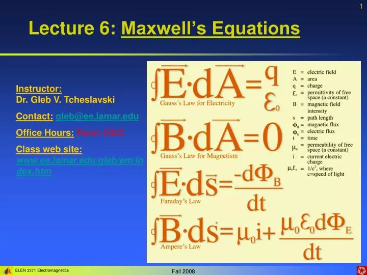
Lecture 6: Maxwell’s Equations. Instructor: Dr. Gleb V. Tcheslavski Contact: gleb@ee.lamar.edu Office Hours: Room 2030 Class web site: www.ee.lamar.edu/gleb/em/Index.htm. Maxwell’s equations.

E N D
Lecture 6: Maxwell’s Equations Instructor: Dr. Gleb V. Tcheslavski Contact:gleb@ee.lamar.edu Office Hours:Room 2030 Class web site:www.ee.lamar.edu/gleb/em/Index.htm
Maxwell’s equations The behavior of electric and magnetic waves can be fully described by a set of four equations (which we have learned already). Faraday’s Law of induction (6.2.1) Ampere’s Law (6.2.2) (6.2.3) Gauss’s Law for electricity Gauss’s Law for magnetism (6.2.4)
Maxwell’s equations And the constitutive relations: (6.3.1) (6.3.2) (6.3.3) They relate the electromagnetic field to the properties of the material, in which the field exists. Together with the Maxwell’s equations, the constitutive relations completely describe the electromagnetic field. Even the EM fields in a nonlinear media can be described through a nonlinearity existing in the constitutive relations.
Maxwell’s equations Integral form Faraday’s Law of induction (6.4.1) Ampere’s Law (6.4.2) (6.4.3) Gauss’s Law for electricity Gauss’s Law for magnetism (6.4.4)
Maxwell’s equations Example 6.1: In a conductive material we may assume that the conductive current density is much greater than the displacement current density. Show that the Maxwell’s equations can be put in a form of a Diffusion equation in this material. We can write: (6.5.1) and, neglecting the displacement current: (6.5.2) Taking curl of (6.5.2): (6.5.3) Expanding the LHS: (6.5.4) The first term is zero and (6.5.5) Is the diffusion equation with a diffusion coefficient D = 1/(0)
Maxwell’s equations Example 6.2: Solve the diffusion equation for the case of the magnetic flux density Bx(z,t) near a planar vacuum-copper interface, assuming for copper: = 0 and = 5.8 x 10⁷ S/m. Assume that a 60-Hz time-harmonic EM signal is applied. Assuming ejt time-variation, the diffusion equation is transformed to the ordinary differential equation: (6.6.1) Where z is the normal coordinate to the boundary. Assuming a variation in the z-direction to be Bx(z) = B0e-z, we write: (6.6.2)
Maxwell’s equations The magnitude of the magnetic flux density decays exponentially in the z direction from the surface into the conductor (6.7.1) where (6.7.2) The quantity = 1/ is called a “skin depth” - the distance over which the current (or field) falls to 1/e of its original value. For copper, = 8.5 mm.
Maxwell’s equations Example 6.3: Derive the equation of continuity starting from the Maxwell’s equations The Gauss’s law: (6.8.1) Taking time derivatives: (6.8.2) From the Ampere’s law (6.8.3) Therefore: (6.8.4) The equation of continuity: (6.8.5)
Poynting’s Theorem It is frequently needed to determine the direction the power is flowing. The Poynting’s Theorem is the tool for such tasks. We consider an arbitrary shaped volume: Recall: (6.9.1) (6.9.2) We take the scalar product of E and subtract it from the scalar product of H. (6.9.3)
Poynting’s Theorem Using the vector identity (6.10.1) Therefore: (6.10.2) Applying the constitutive relations to the terms involving time derivatives, we get: (6.10.3) Combining (6.9.2) and (6.9.3) and integrating both sides over the same v…
Poynting’s Theorem (6.11.1) Application of divergence theorem and the Ohm’s law lead to the PT: (6.11.2) Here (6.11.3) is the Poynting vector – the power density and the direction of the radiated EM fields in W/m2.
Poynting’s Theorem The Poynting’s Theorem states that the power that leaves a region is equal to the temporal decay in the energy that is stored within the volume minus the power that is dissipated as heat within it – energy conservation. EM energy density is (6.12.1) Power loss density is (6.12.2) The differential form of the Poynting’s Theorem: (6.12.3)
Poynting’s Theorem Example 6.4: Using the Poynting’s Theorem, calculate the power that is dissipated in the resistor as heat. Neglect the magnetic field that is confined within the resistor and calculate its value only at the surface. Assume that the conducting surfaces at the top and the bottom of the resistor are equipotential and the resistor’s radius is much less than its length. The magnitude of the electric field is (6.13.1) and it is in the direction of the current. The magnitude of the magnetic field intensity at the outer surface of the resistor: (6.13.2)
Poynting’s Theorem The Poynting’s vector (6.14.1) is into the resistor. There is NO energy stored in the resistor. The magnitude of the current density is in the direction of a current and, therefore, the electric field. (6.14.2) The PT: (6.14.3) (6.14.4) The electromagnetic energy of a battery is completely absorbed with the resistor in form of heat.
Poynting’s Theorem Example 6.5: Using Poynting’s Theorem, calculate the power that is flowing through the surface area at the radial edge of a capacitor. Neglect the ohmic losses in the wires, assume that the radius of the plates is much greater than the separation between them: a >> b. Assuming the electric field E is uniform and confined between the plates, the total electric energy stored in the capacitor is: (6.15.1) The total magnetic energy stored in the capacitor is zero.
Poynting’s Theorem The time derivative of the electric energy is (6.16.1) This is the only nonzero term on the RHS of PT since an ideal capacitor does not dissipate energy. We express next the time-varying magnetic field intensity in terms of the displacement current. Since no conduction current exists in an ideal capacitor: (6.16.2) Therefore: (6.16.3)
Poynting’s Theorem The power flow would be: (6.17.1) In our situation: (6.17.2) and (6.17.3) Therefore: (6.17.4) We observe that (6.17.5) The energy is conserved in the circuit.
Time-harmonic EM fields Frequently, a temporal variation of EM fields is harmonic; therefore, we may use a phasor representation: (6.18.1) (6.18.2) It may be a phase angle between the electric and the magnetic fields incorporated into E(x,y,z) and H(x,y,z). Maxwell’s Eqn in phasor form: (6.18.3) (6.18.4) (6.18.5) (6.18.6)
Time-harmonic EM fields Power is a real quantity and, keeping in mind that: (6.19.1) complex conjugate Since (6.19.2) Therefore: (6.19.3) Taking the time average, we obtain the average power as: (6.19.4)
Time-harmonic EM fields Therefore, the Poynting’s theorem in phasors is: (6.20.1) Total power radiated from the volume The energy stored within the volume The power dissipated within the volume Indicates that the power (energy) is reactive
Time-harmonic EM fields Example 6.6: Compute the frequency at which the conduction current equals the displacement current in copper. Using the Ampere’s law in the phasor form, we write: (6.21.1) Since (6.21.2) and (6.21.3) Therefore: (6.21.4) Finally: (6.21.5) At much higher frequencies, cooper (a good conductor) acts like a dielectric.
Time-harmonic EM fields Example 6.7: The fields in a free space are: (6.22.1) Determine the Poynting vector if the frequency is 500 MHz. In a phasor notation: (6.22.2) And the Poynting vector is: (6.22.3) HW 5 is ready
What is diffusion equation? The diffusion equationis a partial differential equation which describes density fluctuations in a material undergoing diffusion. Diffusion is the movement of particles of a substance from an area of high concentration to an area of low concentration, resulting in the uniform distribution of the substance. Similarly, a flow of free charges in a material, where a charge difference between two locations exists, can be described by the diffusion equation. Back