Download
1 / 97
970 likes | 977 Views
This paper introduces SEEDEEP, a deep web search tool that supports online structured queries in real-time. It addresses challenges in integration, searching, and performance, and proposes novel sampling and stratification techniques for accurate and efficient query processing.

E N D
SEEDEEP: A System for Exploring and Querying Deep Web Data Sources Fan Wang Advisor: Prof. Gagan Agrawal Ohio State University
The Deep Web • The definition of “the deep web” from Wikipedia The deep Web refers to World Wide Web content that is not part of the surface web, which is indexed by standard search engines. • Some Examples: Expedia, Priceline
The Deep Web is Huge and Informative • 500 times larger than the surface web • 7500 terabytes of information (19 terabytes in the surface web) • 550 billion documents (1 billion in the surface web) • More than 200,000 deep web sites • Relevant to every domain: scientific, e-commerce, market • 95 percent of the deep web is publicly accessible (with access limitations)
How to Access Deep Web Data 1. A user issues query through input interfaces of deep web data sources 3. Trigger search on backend database 2. Query is translated into SQL style query Select price From Expedia Where depart=CMH and arrive=SEA and dedate=“7/13/10” and redate=“7/16/10” 4. Answers returned through network
Drawbacks • Constrained flexibility • Types of queries: aggregation query, nested query, queries with grouping requirement • User specified predicates • Inter-dependent data sources • Users may want data from multiple correlated data sources • Long latency • Network transmission time • Denial of service
Goal Develop a deep web search tool which could support online (real time) structured, and high level queries (semi)automatically
Challenges • Challenges for Integration • Self-maintained and created • Heterogeneous, hidden and dynamically updated metadata • Challenges for Searching • Limited data access pattern • Data redundancy and data quality • Data source dependency • Challenges for Performance • Network latency • Fault tolerance issue
Our Contributions (1) • Support online aggregation over deep web • Answer deep web aggregation search in a OLAP fashion • Propose novel sampling techniques to find accurate approximate answers in a timely manner • Support low selectivity query over deep web • Answer low selectivity query in presence of limited data access • Propose a novel Bayesian method to find optimal stratification for hidden selective attribute
Our Contributions (2) • Support structured SQL queries over the deep web • Support SPJ, aggregation, and nested queries • Automatic hidden schema mining • A statistic framework to discover hidden metadata from deep web data sources • Novel query caching mechanism for query optimization • Effective fault tolerance handling mechanism
System Overview Sampling the deep web Online aggregation Low selectivity query Hidden schema discovery Data source integration Structured SQL query
Outline • Introduction • Sampling methods for online aggregation query • Motivation • ANS and TPS methods • Evaluation • Stratification methods for low selectivity query • Motivation • Harmony search and Bayesian based adaptation • Evaluation • Future work and conclusion
Online Aggregation Motivation • Aggregation queries requiring data enumeration I want to know the average airfare from US to Europe across all major US airline flights in the next week Deep Web Data Source Relational Database AA: 500 UA: 550 NYC, London Select AVG(airfare) From AirTable AT Where AT.depart=any US city and AT.arrive=any European city USAir: 450 Delta: 400 Boston, Paris UA: 600 AA: 650 LA, Rome Need Enumeration!!! Where do you get these names? How long can you wait? What if the data is updated dynamically?
Initial Thoughts • Sampling: Approximate answers • Simple random sampling (SRS) • Every data record has the same probability to be selected • Drawbacks of SRS • Bad performance on skewed data • High sampling cost to perform SRS on deep web (Dasgupta et al, HDSampler)
We Want To Achieve • Handle data with (probably high) skew • Top 20 IT companies account for 80% of the sales among all top 100 IT companies in 2005 • Hidden data (hard to gather statistical information) • Has skew or not? • Unknown data distribution • Pilot sample, how much can you trust your pilot sample? • Lower sampling cost for sampling deep web data
Our Contributions • Two Sampling Algorithms • ANS (Adaptive Neighborhood Sampling): handling skewed data, sample skew causing data easier • TPS (Two Phase adaptive Sampling): lower sampling cost • Performance • Accurate estimates without prior knowledge • ANS and TPS outperform HDSampler by a factor of 4 on skewed data • TPS has one-third of the sampling cost of HDSampler
Background Knowledge Associated Samples A survey on a type of rare monkey, which only lives in a small but dangerous area in southern China
Why this is good and Can we use it? • Sample more rare but significant data records • Good for handling with skewed data • Associated samples have relatively low sampling cost • Cheaper than SRS with the same sample size • Yes, we can use it! ~~ with modification • Much real world data has skew (IT company, household income) • Rare data often form clusters • Deep web data sources often return multiple records w.r.t. one input sample
Drawbacks • Performance depends on the initial sample • Initial sample is simple random sample • No cost limit explicitly considered • What is the size of the initial sample? • How many associated samples should be added?
The ANS Sampling Algorithm • Select a random sample • Stop random sampling if any of the two termination rules applies • We have sampled k number of units of interest • We have reached the cost limit • Take the sampled data record, add it to our sample • If this data record is a unit of interest • Obtain its neighbors (neighborhood sampling) • For each data records obtained from neighborhood sampling • Add it to our sample • Perform recursive neighborhood sampling if necessary • If neighborhoods are too large • Increase unit of interest threshold • If neighborhoods are too small • Decrease unit of interest threshold Aggressively sample skew causing data Control sampling cost
ANS Example • Estimate the total sale of IT companies in 2005 • Each point represents a company’s sale record • Color shows the scale of the sale value, the darker, the higher • Neighborhood of data records is defined according to some rules
Unit of interest: sales larger than a threshold • Select initial random samples • sequentially until we have k units • of interest (k=3) 2. Explore the neighborhood recursively for all units of interest until the total number of samples reach a limit 3. If too many neighbors are Included, we increase the threshold of unit of interest
Estimators and Analysis for ANS • Estimator for AVG, fixed unit of interest threshold β is the percentage of units of Interest w.r.t. entire data set β=(k-1)/(n-1) Lemma 1: The above estimator is a biased estimator, when k is small, the bias is very small • We also proposed estimator for variable unit of interest threshold using post-stratification is the estimated average value from the hth stratum (all samples corresponding to one specific unit of interest threshold value)
Drawbacks of ANS • Initial samples are simple random samples • SRS: one input search only gets one sample from the output page • High cost
The TPS Sampling Algorithm Aggressively draw skew Causing data • Partition data set D into M sub-spaces • According to combinations of input attribute values • Random select m sub-spaces • Select a sample of size n1 from each of the m selected sub-spaces • First phase sampling • For one selected sub-space, if any such selected data record is a unit of interest, proceed • Select a sample of size n2 from the corresponding sub-spaces • Second phase sampling • Sub-spaces contains units of interest in the first sampling phase may give us more units of interests in the second sampling phase Low sampling cost
Unit of interest: sales larger than a threshold • Random select the sub • spaces (input search) 2. Random select N1 samples In each selected subspace N1=4 3. If any sample selected in a sub space is a unit of interest, select N2 samples from the sub space again, N2=3
Evaluation • Data sets • Synthetic data sets: generated using MINITAB, varying data skew from 1 to 9 • US Census data: 2002 US economic census data on wholesale trade product lines listed by the kind of business (skew=8) • Yahoo! Auto: prices of used Ford cars from 2000 to 2009 located within 50 miles of a zipcode (skew=0.7) • Metrics • AER: Absolute Error Rate • Sampling cost: number of input samples needed • Methods • ANS • TPS • SRS
ANS Performance w.r.t. Data Skew 1. AER increases moderately with the increase of data skew 2. When k=8, AER is consistently smaller than 19% 3. Larger k doesn’t help much to improve
TPS Performance w.r.t. Data Skew 1. With the increase of data skew, AER increases moderately 2. For sub-space sample size of 30%, AER always smaller than 17%
AER Comparison on Synthetic Data 1. All methods work well on small skew data 2. HDSampler has bad performance on data with skew>2 3. Our two methods outperform HDSampler by a factor of 5
AER Comparison on Yahoo! Data 1. For AVG, three methods are comparable in terms of accuracy 2. For MAX, our methods are better (by a factor of 4)
Sampling Cost Comparison on Yahoo Data More Results 1. To achieve a low AER, TPS has one-third of the sampling cost of HDSampler 2. The total number of samples TPS obtained (with same cost in time) is twice the number of samples HDSampler obtained
Outline • Introduction • Sampling methods for online aggregation query • Motivation • ANS and TPS methods • Evaluation • Stratification methods for low selectivity query • Motivation • Harmony search and Bayesian based adaptation • Evaluation • Future work and conclusion
Motivating Example: Low Selectivity • Random Sampling • None of the selected records satisfies the low selectivity predicate • Stratified Sampling • Partitioning attribute, selective attribute • How to perform stratification • Distance based methods (clustering, outlier indexing) • Selective attribute is not queriable • Auxiliary attribute based stratification • Dalenius and Hodges’s method, Ekman’s method, Gunning and Horgan’s geometric method • Require strong correlation between auxiliary and selective attribute
Our Contributions • We focus on queries in the following format • Propose a Bayesian adaptive harmony search stratification method to stratify a hidden selective attribute based on an auxiliary attribute • The stratification accurately reflects the distribution of the hidden selective attribute when correlation is weak • Estimations from our stratification outperforms existing methods by a factor of 5 • Estimation accuracy obtained from our method is higher than 95% for 0.01% selectivity queries
Background: Stratification • Purpose • Within stratum homogeneity • Partition data set R into k strata • Partitioning attribute x has value range , find k-1 breaking points • Sampling allocation • Neyman allocation • Bayesian Neyman allocation
Background: Harmony Search (1) • A phenomenon-mimicking meta-heuristic algorithm inspired by the improvisation process of musicians • Optimize an objective function • Initialize the harmony memory, M random guesses of the decision variable vector
Background: Harmony Search (2) • Improvise a new harmony from the harmony memory • A new harmony vector is generated from two parameters HMCR and PAR. • Update harmony memory • Termination
Algorithm Overview (1) • Find the best stratification of the selective attribute 2.1 0 0.85 0 0.45 0.75 1.1 0.45 1.4 2.1
Algorithm Overview (2) • Consider an auxiliary attribute as the partitioning attribute • Harmony memory • A list of breaking points vectors of the auxiliary attribute
Harmony Objective Function • What is a good stratification? • Condition 1: homogenous data within stratum • Small sample variance summation across strata • Condition 2: stratification with high precision, i.e., the low selective region of the distribution is exclusively covered by some strata
Sample Allocation • Determine the number of samples assigned to each stratum • What stratum should be put heavier sampling weight? • Stratum with diversity (more heterogeneous) • High sample variance • Stratum which covers large percentage of the low selective region • High precision
Parameter Adaptation: Overview • Two parameters: HMCR and PAR X: value of HMCR parameter Y: precentage of cases in which we obtain better harmony vector
Bayesian Method Overview • Estimate unknown parameter (posterior distribution) based on prior knowledge or belief (prior distribution) • Observed data y, unknown parameter θ • In our scenario • Observed data: the harmony parameter values which yield better harmony vector • Unknown parameter: adaptation pattern of harmony parameters
Bayesian Adaptation (1) • Assume the adaptation patterns of parameters HMCR and PAR follows probability functions • Represent our belief in θ as a prior probability distribution • Observe our data: the HMCR and PAR parameters which yield the best new harmony vector based on the current harmony memory, denoted as • Based on , compute θ (posterior distribution), denoted as (Details) • Compute the adapted parameter value as
Bayesian Adaptation (2) • Probability function • Prior distribution of θ Details
Evaluation • Data sets • Synthetic data sets: generated using MINITAB, varying correlation between auxiliary attribute and selective attribute from 1 to 0.3 • US Census data, correlation (number of settlements and sale) 0.56 • Yahoo! Auto, correlation (year and mileage) 0.7 • Metric • AER: Absolute Error Rate • Methods • Leaps and Bounds (L&B) • Dalenius and Hodges (D&H) • Random Sampling (No Stratification) • Ours (HarmonyAdp)
HarmonyAdp Performance (1) 1. Higher accuracy with more iterations 2. Iteration>40 (2% of total data size), low AER for all selectivity values 3. Robust with respect to data correlation
Four Methods Comparison (1) 1. All methods work well on easy queries 2. When queries get harder, D&H, L&B and Random degrade severely. Ours has good performance 3. For 0.1% queries, our method outperforms others by a factor of 5 4. For extreme low selectivity queries, the error rate from our method is always lower than 18%