Download
1 / 73
730 likes | 827 Views
Programming Sensor Networks. David Gay Intel Research Berkeley. Object tracking Sensors take magnetometer readings, locate object using centroid of readings Communicate using geographic routing to base station Robust against node and link failures. Environmental monitoring

E N D
Programming Sensor Networks David Gay Intel Research Berkeley
Object tracking • Sensors take magnetometer readings, locate object using centroid of readings • Communicate using geographic routing to base station • Robust against node and link failures
Environmental monitoring • Gather temperature, humidity, light from a redwood tree • Communicate using tree routing to base station • 33 nodes, 44 days
Challenges and Requirements • Expressivity • Many applications, many OS services, many hardware devices • Real-time requirements • Some time-critical tasks (sensor acquisition and radio timing) • Constant hardware evolution • Reliability • Apps run for months/years without human intervention • Extremely limited resources • Very low cost, size, and power consumption • Reprogrammability • “Easy” programming • used by non-CS-experts, e.g., scientists
Recurring Example • Multi-hop data collection • Motes form a spanning tree rooted at a base station node • Motes periodically sample one or more sensors • Motes perform some local processing, then send sensor data to parent in tree • Parents either process receiveddata (aggregation) or forwardit as is
Programming the Hard Way C compiler Assembler
“The Real Programmer’s” Scorecard • Expressivity • Real-time requirements • Constant hardware evolution • Reliability • Extremely limited resources • Reprogrammability • “Easy” programming
Programming the Hard Way C compiler Assembler
3 Practical Programming Systems • nesC • A C dialect designed to address sensor network challenges • Used to implement TinyOS, Maté, TinySQL (TinyDB) • Maté • An infrastructure for building virtual machines • Provide safe, efficient high-level programming environments • Several programming models: simple scripts, Scheme, TinySQL • TinySQL • A sensor network query language • Simple, well-adapted to data-collection applications
Component-based C dialect All cross-component interaction via interfaces Connections specified at compile-time Simple, non-blocking execution model Tasks Run-to-completion Atomic with respect to each other Interrupt handlers Run-to-completion “Whole program” Reduced expressivity No dynamic allocation No function pointers nesC overview
nesC component model • interface Init { • command bool init(); • } • module AppM { • provides interface Init; • uses interface ADC; • uses interface Timer; • uses interface Send; • } • implementation { • … • } A call to a command, such as: bool ok = call Init.init(); is a function-call to behaviour provided by some component (e.g., AppM).
nesC component model • interface Init { • command bool init(); • } • module AppM { • provides interface Init; • uses interface ADC; • uses interface Timer; • uses interface Send; • } • implementation { • … • } • interface ADC { • command void getData(); • event void dataReady(int data); • } Interfaces are bi-directional. AppM can call ADC.getData and must implement event void ADC.dataReady(int data) { … } The component to which ADC is connected will signaldataReady, resulting in a function-call to ADC.dataReady in AppM.
nesC component model • interface Init { • command bool init(); • } • module AppM { • provides interface Init; • uses interface ADC; • uses interface Timer; • uses interface Send; • } • implementation { • TOS_Msg myMsg; • int busy; • event void ADC.dataReady() • { • call Send.send(&myMsg); • busy = TRUE; • } • ... • } • interface ADC { • command void getData(); • event void dataReady(int data); • } • interface Timer { • command void setRate(int rate); • event void fired(); • } • interface Send { • command void send(TOS_Msg *m); • event void sendDone(); • }
nesC component model • configuration App { } • implementation { • } • components Main, AppM, TimerC, Photo, MessageQueue; • Main.Init -> AppM.Init; • AppM.Timer -> TimerC.Timer; • Main.Init -> TimerC.Init; • … • module AppM { • provides interface Init; • uses interface ADC; • uses interface Timer; • uses interface Send; • } … Main Init Init AppM Timer ADC Send Init Timer ADC Send TimerC Photo MessageQueue
Some Other Features • Parameterised interfaces, generic interfaces • interface ADC[int id]: runtime dispatch between interfaces • interface Attribute<t>: type parameter to interface • Generic components (allocated at compile-time) • Reusable components with arguments: generic module Queue(typedef t, int size) … • Generic configurations can instantiate many components at once • Distributed identifier “allocation” • unique(“some string”): returns a different number at each use with the same string, from a contiguous sequence starting at 0 • uniqueCount(“some string”): returns the number of uses of unique(“some string”) • Concurrency support • Atomic sections, compile-time data-race detection
nesC Scorecard • Expressivity • Subsystems: radio stack, routing, timers, sensors, etc • Applications: data collection, TinyDB, Nest final experiment, etc • Constant hardware evolution • René Mica Mica2 MicaZ; Telos (x3) • Many other platforms at other institutions • How was this achieved? • The component model helps a lot, especially when used following particular patterns
nesC Scorecard • Expressivity • Subsystems: radio stack, routing, timers, sensors, etc • Applications: data collection, TinyDB, Nest final experiment, etc • Constant hardware evolution • René Mica Mica2 MicaZ; Telos (x3) • Many other platforms at other institutions • How was this achieved? • The component model helps a lot, especially when used following particular patterns • Placeholder: allow easy, application-wide selection of a particular service implementation • Adapter: adapt an old component to a new interface
Placeholder:allow easy, application-wide selection of a particular service implementation Main Init Router ReliableRoute MRoute Data Collection Route Management • Motivation • services have multiple compatible implementations • routing ex: MintRoute, ReliableRoute; hardware independence layers • used in several parts of system, application • ex: routing used in network management and data collection • most code should specify abstract service, not specific version • application selects implementation in one place
Placeholder:allow easy, application-wide selection of a particular service implementation Init Router Route Main MRoute Data Collection Management • configuration Router { • provides Init; • provides Route; • uses Init as XInit; • uses Route as XRoute; • } implementation { • Init = XInit; • Route = XRoute; • } • configuration App { } • implementation { • components Router, MRoute; • Router.XInit -> MRoute.Init; • Router.XRoute -> MRoute.Route; • … • }
Adapter:adapt an old component to a new interface • Motivation • functionality offered by a component with one interface needed needs to be accessed by another component via a different interface. Light AttrPhoto TinyDB ADC Attribute
Adapter:adapt an old component to a new interface Light AttrPhoto TinyDB ADC Attribute • generic module AdaptAdcC • (char *name, typedef t) { • provides Attribute<t>; • provides Init; • uses ADC; • } implementation { • command void Init.init() { • call Attribute.register(name); • } • command void Attribute.get() { • call ADC.get(); • } • … • } • configuration AttrPhoto { • provides Attribute<long>; • } • implementation { • components Light, • new AdaptAdcC(“Photo”, long); • Attribute = AdaptAdcC; • AdaptAdcC.ADC -> Light; • }
nesC scorecard • Expressivity • Constant hardware evolution • Real-time requirements (soft only) • Radio stack, especially earlier bit/byte radios • Time synchronisation • High-frequency sampling • Achieved through • Running a single application • Having full control over the OS (cf Placeholder)
nesC scorecard • Expressivity • Constant hardware evolution • Real-time requirements (soft only) • Reliability • C is an unsafe language • Concurrency is tricky • Addressed through • A static programming style, e.g., the Service Instance pattern • Compile-time checks such as data-race detection
Service Instance:support multiple instances with efficient collaboration Data Collection Timer timer0 Clock Radio timer1 timer2 MRoute • Motivation • multiple users need independent instance of service • ex: timers, file descriptors • services instances need to coordinate, e.g., for efficiency • ex: n timers sharing single underlying hardware timer
Service Instance:support multiple instances with efficient collaboration Data Collection Timer timer0 Clock Radio timer1 • module TimerP { • provides Timer[int id]; • uses Clock; • } • implementation { • timer_t timers[uniqueCount(“Timer”)]; • command Timer.start[int id](…) { … } • } • generic configuration TimerC() { • provides interface Timer; • } • implementation { • components TimerP; • Timer = TimerP.Timer[unique(“Timer”)]; • } • components Radio, TimerC; • Radio.Timer –> new TimerC();
Race condition example • module AppM { … } • implementation { • bool busy; • async event void Timer.fired() { • // Avoid concurrent data collection attempts! • if (!busy) { // Concurrent state access • busy = TRUE; // Concurrent state access • call ADC.getData(); • } • } • … • }
Data race detection • Every concurrent state access is a potential race condition • Concurrent state access: • If object O is accessed in a function reachable from an interrupt entry point, then all accesses to O are potential race conditions • All concurrent state accesses must occur in atomic statements • Concurrent state access detection is straightforward: • Call graph fully specified by configurations • Interrupt entry points are known • Data model is simple (variables only)
Data race fixed • module AppM { … } • implementation { • bool busy; • async event void Timer.fired() { // From interrupt • // Avoid concurrent data collection attempts! • bool localBusy; • atomic { • localBusy = busy; • busy = TRUE; • } • if (!localBusy) • call ADC.getData(); • }
nesC scorecard • Expressivity • Constant hardware evolution • Real-time requirements (soft only) • Reliability • Extremely limited resources • Complex applications exist: NEST FE, TinyScheme, TinyDB • Lifetimes of several months achieved • How? • Language features: resolve “wiring” at compile-time • Compiler features: inlining, dead-code elimination • And, of course, clever researchers and hackers
Resource Usage • An interpreter specialised for data-collection • Makes heavy use of components, patterns • Optimisation reduces power by 46%, code size by 44% • A less component-intensive system (the radio) “only” gains 7% from optimisation
nesC scorecard • Expressivity • Constant hardware evolution • Real-time requirements (soft only) • Reliability • Extremely limited resources • Reprogrammability • Whole program only • Provided by a TinyOS service
nesC scorecard • Expressivity • Constant hardware evolution • Real-time requirements (soft only) • Reliability • Extremely limited resources • Reprogrammability • “Easy” programming • Patterns help, but… • Split-phase programming is painful • Distributed algorithms are hard • Little-to-no debugging support
3 Practical Programming Systems • nesC • A C dialect designed to address sensor network challenges • Used to implement TinyOS, Maté, TinySQL (TinyDB) • Maté • An infrastructure for building virtual machines • Provide safe, efficient high-level programming environments • Several programming models: simple scripts, Scheme, TinySQL • TinySQL • A sensor network query language • Simple, well-adapted to data-collection applications
The Maté Approach • Goals: • Support reprogrammability, nicer programming models • While preserving efficiency and increasing reliability • Sensor networks are application specific. • We don’t need general programming: nodes in redwood trees don’t need to locate snipers in Sonoma. • Solution: an application specific virtual machine (ASVM). • Design an ASVM for an application domain, exposing its primitives, and providing the needed flexibility with limited resources..
The Maté Approach • Reprogrammability • Transmit small bytecoded programs. • Reliability • The bytecodes perform runtime checks. • Efficiency • The ASVM exposes high-level operations suitable to the application domain. • Support a wide range of programming models, applications • Decompose an ASVM into a • core, shared template • programming model and application domain extensions
ASVM Architecture Template Program Store Scheduler Concurrency Manager Operations Handlers
ASVM Template • Threaded, stack-based architecture • One basic type, 16-bit signed integers • Additional data storage supplied by language-specific operations • Scheduler • Executes runnable threads in a round-robin fashion • Invokes operations on behalf of handlers • Concurrency Manager • Analyses handler code for shared resources (conservative, flow insensitive, context insensitive analysis). • Ensures race free and deadlock free execution • Program Store • Stores and disseminates handler code
ASVM Extensions • Handlers: events that trigger execution • One-to-one handler/thread mapping (but not required) • Examples: timer, route forwarding request, ASVM boot • Operations: units of execution • Define the ASVM instruction set, and can extend an ASVM’s set of supported types as well as storage. • Two kinds: primitives and functions • Primitives: language dependent (e.g., jump, read variable) • Can have embedded operands (e.g., push constant) • Functions: language independent (e.g., send()) • Must be usable in any ASVM
Maté scorecard • Expressivity • By being tailored to an application domain
Maté scorecard • Expressivity • Real-time requirements • Just say no!
Maté scorecard • Expressivity • Real-time requirements • Just say nesC!
Maté scorecard • Expressivity • Real-time requirements • Constant hardware evolution • Presents a hardware-independent model • Relies on nesC to implement it
QueryVM: an ASVM • Programming Model • Scheme program on all nodes • Application domain • multi-hop data collection • Libraries • sensors, routing, in-network aggregation • QueryVM size: • 65 kB code • 3.3 kB RAM
QueryVM Evaluation • Simple: collect light from all nodes every 50s • 19 lines, 105 bytes
Simple query • // SELECT id, parent, light INTERVAL 50 • mhop_set_update(100); settimer0(500); mhop_set_forwarding(1); • any snoop() heard(snoop_msg()); • any intercept() heard(intercept_msg()); • any heard(msg) snoop_epoch(decode(msg, vector(2))[0]); • any Timer0() { • led(l_blink | l_green); • if (id()) { • next_epoch(); • mhopsend(encode(vector(epoch(), id(), parent(), light()))); • } • }
QueryVM Evaluation • Simple: collect light from all nodes every 50s • 12 lines, 105 bytes • Conditional: collect exponentially weighted moving average of temperature from some nodes • 32 lines, 167 bytes • SpatialAvg: compute average temperature, in-network • 31 lines, 127 bytes • or, 117 lines if averaging code in Scheme
Maté scorecard • Expressivity • Real-time requirements • Constant hardware evolution • Reliability • Runtime checks • Reprogramming always possible
Maté scorecard • Expressivity • Real-time requirements • Constant hardware evolution • Reliability • Extremely limited resources • VM expresses application logic in high-level operations • But, don’t try and write an FFT!
Ran queries on 42 node network Compared QueryVM to nesC implementation of same queries Fixed collection tree and packet size to control networking cost. QueryVM Energy • QueryVM sometimes uses less energy than the nesC code. • Due to vagaries of radio congestion (nesC nodes all transmitting in synch) • Decompose QueryVM cost using a 2-node network. • Run with no query: base cost (listening for messages). • Ran programs for eight hours, sampling power draw at 10KHz • No measurable energy overhead! • There’s not much work in the application code…
Maté scorecard • Expressivity • Real-time requirements • Constant hardware evolution • Reliability • Extremely limited resources • Reprogramming • Enough said already…