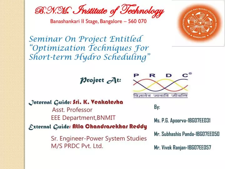
B.N.M . Institute of Technology Banashankari II Stage, Bangalore – 560 070

1. B.N.M.InstituteofTechnology Banashankari II Stage, Bangalore – 560 070 Seminar On Project Entitled “Optimization Techniques For Short-term Hydro Scheduling” Project At: Internal Guide:Sri. K. Venkatesha Asst. Professor EEE Department,BNMIT By: Ms. P.G. Apoorva-1BG07EE031 Mr. Subhashis Panda-1BG07EE050 Mr. Vivek Ranjan-1BG07EE057 External Guide:Atla Chandrasekhar Reddy Sr. Engineer-Power System Studies M/S PRDC Pvt. Ltd.

2. INTRODUCTION: • The aim is to schedule hydrogeneration for a period of 1day to 1 week for better reliable and economic operation of power system. • Types Of Hydroscheduling: • Long Term Scheduling(1week-3years) • Short Term Scheduling(1day-1week) • The objective of the short-term hydro scheduling program is to maximize the value of thestored energy in thereservoirs at theend of the study, which is equivalent tominimizing thevalue of the water flows through turbines and spillways. • Short-range hydro-scheduling (1 day to I wk) involves the hour-by-hour scheduling of all generation on a system to achieve minimum production cost for the given time period.

3. Real Time Input Obtained From Power System Power System Problem Formulation Tool Optimization Tool Optimized Output

4. Various Aspects Of Scheduling: • Hydro+Thermal=Demand. • Scheduling Plays an vital role in power system reliabilty. • Cost Of Thermal production is v.high compared to Hydro. Fig. 1– Total hourly hydro and thermal power production

5. Water Inflow Long Term Hydroscheduling Hydro Scheduling Short Term Hydrothermal Co-ordination Thermal Unit Commitment OPF(Optimal Power Flow)

6. PROBLEM FORMULATION: Objective function • Cost Function • Fuel Availability Power System Model Thermal Constraints • Water Balance Equation • Storage & Discharge limitations • Power Production • Spill Characteristics • System Constraints Hydro

7. KALINADI HYDRO ELECTRIC PROJECT- FLOW CHART

9. Objective Function: Thermal Cost Function:- Psj = The steam plant net output at time period j. Sfk = The slopes of the piecewise linear steam-plant cost function. FIG. 2 Steam plant piecewise linear cost function Considering Two Thermal Units, The Objective function is: Minimize,F=∑ ∑ fij+ds1+Srs1 Where: ds1 & Srs1 are the slack variables for demand and spinning reserve. i=No. of units. j=No of periods.

10. Hydro Constraints: 1)Water Balance Equation: • Water inflow(A) • Discharge(Q) • Spillage(S) • Volume Of Water In The Resorvoir(V) • Irrigation(I) • Time Delay(Important Consideration) For Example, Let’s consider Resorvoir 7, At the end Of 1st hour: V71+S71+Q71=V70 +A71-I71 At the end Of 5th hour: V75-V74-S52-S43-Q61-Q52+S75+Q75=A75-I75 Explains Time Delay

11. 2)Storage & Discharge Limitations: • Initial Volume • Final Volume • Discharge Amount • Considering Resorvoir 2 i.e.(SUPA DAM): • V21 to V223=(55-4190 Million Cubic meter) • V20 & V224=(2178 Million Cubic meter) • Q2=Q3,Q7=Q8,Q9=Q10 • Considering Plant3 i.e.(SUPA),the Discharge Limit is: • Q3=(0-154) For All T. • Similarly For plant 10 i.e.(Kadra),the Discharge Limit is: • Q10=(0-527) For All T.

12. 3)Hydro Power Production: Fig. 3.Typical I/O function for a hydro plant with three units. • The Characteristics Shows: • P=KQ ;Where ,P=Hydro Generation, • K=slope • Q=Discharge • Considering 3rd Hydro Plant, We can write : • P31=K111*Q311+K112*Q312 • Hence It is written for 2 slope characteristics. • Variable Head study can be implemented in future.

13. 4)Spill Characteristics: • Controlled Spillage • Uncontrolled Spillage FIG. 4 Spill characteristic. The General Equation For Spillage is: Considering Resorvoir 5,The Equation can be written as: S51=V511*0+V512*.12+V513*.2 i.e 10-20% of the volume is considered for spilling action.

14. 5)System Constraints: • 1)Generation-Demand Balance Equation. • Hydro + Thermal=Demand • 2)Spinning Reserve • To meet unexpected demand or forecast. • To meet unexpected generation failure. • The Equation For 1st Hour is: • P31+P61+P81+P101+G11+G21+ds1=4896(7815*.626488) • Where , • ds1 is a slack variable which takes care of the spinning reserve. • G Is the Thermal Generation.

15. Thermal Constraints: • Thermal Cost Function • Fuel Availability Constraint: For RTPS:1Mw-hr of generation Requires 1.6 tonnes of Fuel. For BTPS:1Mw-hr of generation Requires .64 tonnes of Fuel. Considering Fuel availability as 8000 & 6000 tonnes/day for RTPS and BTPS respectively, The Equations are: 1.6g11+1.6g12+…………..+1.6g124<=8000 (RTPS) .64g21+.64g22+…………...+.64g224<=6000 (BTPS)

16. Why LP? Linear programming is one of the most famous optimization techniques for linear objectives and linear constraints. • Lagrange’s Method: 1)Difficult to add New Constraints 2)Less Flexible 3)More Complex • Dynamic Programming. 1)Time consuming 2)Becomes complex with increased no. of Variables. • Nonlinear Programming. 1)Research & Development On Progress. 2)Can be Implemented in Future. • Linear Programming: 1)Any constraint can be taken care Easily 2)Easier To solve 3)Requires Less time

17. Implemented Algorithms: • Revised Simplex Method Can’t Handle Unbounded Cases. Requires More Time Compared to IP Method. • Upper Bouding Method (Special Case Of Simplex Method) Can Handle Problems With Limits Of Variables. Interior Point methods: • Karmarkar’s Method Requires Initial Feasible Solution (An algorithm is implemented with limitations) Can’t Handle All the LPs. • Dual Affine Variant Method Requires Initial Feasible Solution Can’t Handle All the LPs.

18. Applications: • Linear Programming Can be used for the optimization of: • Short & Long Term Hydro-Scheduling. • Economic Load Dispatch. • Unit Commitment. • Reactive Power Management. • Energy Management System. • Optimal Power Flow. • Apart from Power System Applications, they are used for the Optimization Studies of: • Production Management. • Aircraft Schedules. • Manufacturing Companies. • Resources Management. • And All Other Aspects.

19. Result Analysis: Input:

21. References: