1. Process Mapping

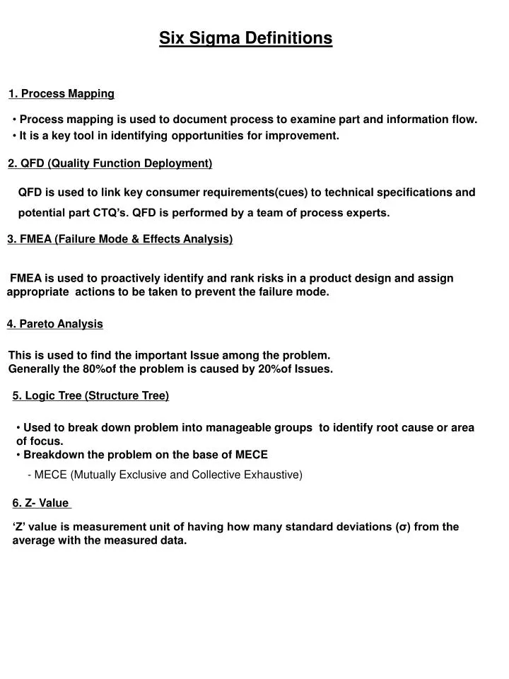
1. Six Sigma Definitions 1. Process Mapping • Process mapping is used to document process to examine part and information flow. • It is a key tool in identifying opportunities for improvement. 2. QFD (Quality Function Deployment) QFD is used to link key consumer requirements(cues) to technical specifications and potential part CTQ’s. QFD is performed by a team of process experts. 3. FMEA (Failure Mode & Effects Analysis) FMEA is used to proactively identify and rank risks in a product design and assign appropriate actions to be taken to prevent the failure mode. 4. Pareto Analysis This is used to find the important Issue among the problem. Generally the 80%of the problem is caused by 20%of Issues. 5. Logic Tree (Structure Tree) • Used to break down problem into manageable groups to identify root cause or area of focus. • Breakdown the problem on the base of MECE - MECE (Mutually Exclusive and Collective Exhaustive) 6. Z- Value ‘Z’ value is measurement unit of having how many standard deviations (σ) from the average with the measured data.

2. 7. Rational Subgroup Regardless of Data types, sample population taken on the short time period and on the condition of homogeneity. 8. Rational Subgrouping Rational subgrouping allows samples to be taken that include only white noise, within the samples. Black noise occurs between the samples. 9. Difference between Long Term and Short Term Process Capability Long Term Capability Short Term Capability • Calculated from data taken over a period • of time long enough that external factors • can influence the process. Ppm defect data • and yield data are, by nature, long-term • measurements. • Zlt (σlt) , Cpk • Need technology and process control for • improvement. • “6σ” means Zlt equals 4.5, Cpk equals 1.5. • Calculated from data taken over a short • enough period of time that there are no • external influences on the process(I.e, • temperature changes, shift changes, operator • changes, raw material lot changes, etc…) • Zst (σst) , Cp • Need technology for improvement. • Process capability on the optimized condition. • “6σ”means Zst equals 6.0, Cp equals 2.0.

3. 10.Repeatability ? Repeatability : “Getting consistent results” ☞ Variation observed with one measurement device when used several times by one operator while measuring the identical characteristic on the same parts. Measure/Re-measure variation 11.Reproducibility ? ☞ Variation obtained from different operators using the same device when measuring the identical characteristic on the same parts. Operator B Operator C Operator A Reproducibility 12. Accuracy ? ☞ The degree of agreement of the measured value to the true magnitude (unbiased values). (Accuracy is typically expressed as 1-%Bias) True (Reference) value Accuracy * Setting a true value is a one that is measured by the most accurate measuring device. Observed average

4. 13. Stability ? Time 1 ☞ Stability is the total variation in the measurements obtained with a measurement system on the same master or reference value when measuring the same characteristic over an extended time period. Stability Time 2 14. Linearity ? ☞ Linearity is the difference in the bias values throughout the expected operating range of the gage. (Gage is less accurate at the low end of specification or operating range than at the high end). LSL USL Actual values Actual values (No Bias) Reference value Reference values Larger Bias Small Bias

5. 15. 1-α = Confidence The probability that can be determined as a right thing when the Null Hypothesis is correct. 16. 1-β = Power of the test The rejecting probability when null Hypothesis you want to test is not right. 17. Chi Square Test This Chi-Square is used to Test hypotheses about the frequency of occurrence of some event happening with equal probability.That is, could this occur by random chance, or is it truly different from what is expected?. 18. Descrete Data Discrete Data: Probability variable which can be counted one by one (Frequency times that come up heads/tails, numbers of defect occurred, sex division, bloodtype division, likes and dislikes, etc.) 19 .ANOVA: ANOVA determines if the variation between the average of the levels is greater than the variation that occurs within the level Avg SS between ANOVA= --------------------- Avg SS within 20. SYSTEMATIC Variation Differences in the measurements which are expected and predictable. EXAMPLE : The summer season is different from the Christmas holidays in the volume of electric range sales. 21. RANDOM Variation Differences in the measurements which are NOT predictable. EXAMPLE: Two refrigerators of the same design, tested for energy usage on two different days, with the same technician, in the same test stand, with the same air temperature, with the same measuring instruments, etc... will probably give two different results.

6. 22. Experimental Design Experimental Design means the active manipulation of independent variables, and observation of the effects on the dependent variables (responses). 23. Interaction Effect An interaction means that the effect of one variable is influenced by the level of another variable. The effect of one variable is not consistent for all levels of the other variables 24. Fractional Factorial Design A DOE which allows for more factors (X’s) to be included in the experimental design for the same number of runs. 25. Highly Fractionated Designs Highly fractionated experiments are experiments where the number of runs is only a little larger than the number of independent variables. Examples: 23-1, 4 runs, 3 independent variables 27-4, 8 runs, 7 independent variables The highly fractionated experiments are useful ONLY for detecting Main Effects. Caution - You can be misled if interactions are large (but this happens infrequently). Statistical tests of significance have less meaning, because there is not a good estimate of the error. You typically look for the relative magnitude of the Main Effects. Highly fractionated experiments are often used for screening, to find the variables that deserve further study. 26. Steps in Planning an Experiment 1) Define the Objective 2) Select the Y Response (Dependent) Variables 3) Select the X (Independent) Variables 4) Choose the X Variable Levels 5) Select the Experimental Design 6) Run the Experiment & Collect the Data 7) Analyze the Data 8) Draw Conclusions 9) Perform Confirmation Run

7. 27. When designing the experiment, consider 10 Key Elements... 1) Orthogonality 2) Randomization 3) Replication 4) Repetition 5) Controls 6) Lurking Variables 7) Noise Variables 8) Blocking 9) Sample Size 10) Confounding 28. Orthogonal arrangements(factorial and fractional factorial test plans) are used to separate the effects of the variables. 29. Randomization to reduce the effects of extraneous variables, and ensure that the statistical tests of significance are valid. Randomize: - Run order - Assignment of experimental units - Measurement order 30. Replication (completely re-setting the experiment and obtaining additional results at the same levels) - Reduces the variability of an estimate (shorter confidence intervals) - Gives an estimate of variation and confidence in the results. 31. Repetition (measure multiple samples from each experimental run) - Not as beneficial as Replication, but does allow you to estimate variation. 32. Controlsand reference distributions. Most experiments are comparative. Including a control or baseline can be extremely useful.

8. 33. Lurking Variablesare variables that can affect the results but are unknown, uncontrolled, uncontrollable or un-measurable. The influence of lurking variables can often be reduced by blocking and randomization. 34. Noise Variablesare known (or thought) to affect the results, but we either cannot or choose not to control them. Examples: humidity, day of the week, competitor incentives. To reduce the effect of noise variables, select test variables that can be monitored across all levels in the experiment. 35. Blocking A Block is group of homogeneous units. Compare independent variables within blocks, not between blocks. Benefits of blocking: • Gives all independent variables an equal chance (a fair test) • Gives some protection against confounding and lurking variables. • Reduces variation and gives higher precision of the estimates. (It is often good to block on time or run order) 36. Determining sample size There is usually a trade-off between cost and precision when deciding how many samples to take. 37. Confounding It is the inability to separate effects of variables from one another, or from interactions. Remember that all fractional factories have some degree of confounding. 38. Confirmation Run The Confirmation Run is necessary to verify that you have truly made improvements. Confirmation Runs should be set up in rational subgroups, similar to process baselining. In effect, you are “Re-baselining” your process at the new settings. 39. Regression A mathematical equation of describing a relationship between the ”Y” and “X’s” Y = b0 + b1x + error where b0 = constant b1 = slope

9. 40. FITSare the predicted values of “Y”calculated from the regression equation for each value of “X” C3 = 0.069 + 0.00383 C1or Predicted Response = 0.069 + 0.00383 (Velocity) 41. RESIDUALS are errors. The presence of residuals demonstrates that the model does not represent the data without mistakes. (Actual Response minus Predicted Response (Fits) for each point). 42. Residual Properties • The average of the Residuals should always be 0.0 • The Residuals should be normally distributed • The Residuals should be randomly distributed. A pattern in the Residuals may indicate • that this model form is incorrect. 43. s:The standard deviation of the residuals (errors). Errors are observed values - expected values. In other words, the distance from the observed points to the fitted line described by the regression equation. (Should be small, for a good model) s = MS(error)1/2 44.R-Sq:The percent of total variation “explained”by the fitted line. The variation accounted for by the factors. (Should be large, for a good model) SSregression SStotal 45.R-Sq(adj):Adjustment for an overfit condition (fitting too many variables into the equation) that incorporates. the number of terms in the model compared to the number of observations R-Sq(adj) = 1 - SSregression / (n-p) SStotal / (n-1) where n = number of observations p = total number of terms in the model R-Sq = * 100

10. 46. Multiple Regression It provides the ability to model the process with either a linear equation or a quadratic equation (an equation with squared terms) 47. Centering We have to “Transform” the related “X’s” variables in order to separate their individual effects on “Y” the transformation method is called ”centering”. Centered data is orthogonal - it allows effects to be separated 48. What are the Pitfalls of Regression? 1. Correlation does not mean causation 2. Fitting the wrong model form 3. Relationships between independent variables (multi-collinearity) 4. Over-fitting; multiple hypothesis tests; too many independent variables 5. Influence of a few extreme values 6. Drawing firm conclusions from passive / happenstance data 49. Limitations of Factorial Designs Two-level factorial experiments cannot be used to estimate curvature. They cannot be used to find an optimum. The relationships between the “Y” and “Xi’s” might involve curves, and might be approximated better with quadratic equations: 50 . Advantages of Central Composite Designs • There are now 5 levels of each independent variable, so there is some ability to detect • departure from a quadratic Model. • The wider range of independent variables gives more precise estimates of the fitted parameters. • If the distance of these Points(α) is chosen such that; α = (number of Cube Points )0.25 (fourth root) then the variance of the predicted response is the same at constant distances from the center of the design. This is called rotatability.

11. Average pure error { } AVERAGE lack of fit 51. Pure error The reproducibility of the response, at constant values of the independent variables. This is the error “Within” (“White noise plus any “Xi’S” not included in the model). 52. Lack-of-fit The deviation of the average from the assumed model. The lack-of-fit will be large if the model does not fit the data well. We need to investigate another model whether this model is fitting properly or not because larger than pure error. • The variation between the 3 open circles is the pure error. • The variation between the average of the 3 • open circles and the fitted line is Lack of fit 53 . Statistical Process Control Enables us to control our process using statistical methods to signal when process adjustments are needed. 54 . Stability Stability also means all subgroup averages and ranges are between their respective control limits and display no evidence of assignable-source (special -cause) variation 55 . R&D Six Sigma The definition of R&D Six sigma is to quantize a consumer’s needs, select CTQ and about selected CTQ, by choosing Tolerance through process capability, is statitical tool to achieve design performance in six sigma level. 56 . CTQ The select few, measurable key characteristics of a specific part/drawing/specification that must be in statistical control to guarantee consumer satisfaction. Therefore, they must be measured and analyzed on-going basis.

12. 57 . QFD This method is to translate Consumer requirements(Voice of consumer) to technical requirements to part CTQ in Product Development Event. 58 . FMEA A process used to identify impact of failure modes from the full array of potential sources 59 . Transfer Function - Classifying a uncertain customer demand quality into System level CTQ. - Classifying a System level CTQ into Subsystem CTQ and then Component Spec. - Classifying a input and output in the user’s situation. - Y=f(x1, x2, x3,…..xn) always define a correlation relation. 60 . System Modeling Types • Mathematical analysis Model : a theoretical correlation figure or physical law for System part. • Motion analysis Model : a description and narration for System function • - Structure analysis Model : dividing a System function into the Components or assigning a efficiency and allowance into Components. 61. Type of a tolerance analysis 1) Nominal & Tolerance (1) Nominal : ● Determining the performance of a product or matching-up dimension on the ideal condition →providing with a datum line that can be considered from a precision analysis. (2)Tolerance : ● A permissive limit dimension ● Being determined with a number ● Being applied at the character of assembly part or unit part. 2) Type (1) Min/Max ● Method that establish the Gap of a System by using the limit tolerance of a contributed parts dimension (2) Root Sum of Square(RSS) ● Statistical method that establish the capability of a System on the basis of a System dimension and part capability.

13. 62 . Difference between RSS and Monte Carlo Mathod RSS method RSS is correct, more fast and easier. RSS is used when a equation is linear and have a probability. (Gap = A + ∑BiXi, here Bi is a constant, Xi is a size(dimension) of part.) Monte Carlo method Monte Carlo is used in System with a non-Linear occasion. Monte Carlo method isn’t perfect but the more frequent of test, get the closer result of test. An encouraged simulation frequency: When initial estimate and repeat occasion, n = 100 for a initial decision, n = 10,000. Using the Minitab, we can do Monte Carlo analysis.