Download
1 / 30
300 likes | 398 Views
NEMS/GFS Modeling Summer School 2013 Radiation. Yu-Tai Hou. About the Course. - Will not focus on basic theory (covered in classical physics courses), and neither will explore in depth of the cutting-edge research topics (diverse, interdisciplinary, unsettled)

E N D
About the Course - Will not focus on basic theory (covered in classical physics courses), and neither will explore in depth of the cutting-edge research topics (diverse, interdisciplinary, unsettled) - Will focus on the main structure and practical usage of the model for controlled experiments Outlines: 1. The role of radiative process in NWP and the difficulties for seeking efficient solutions 2. Evolution of radiation packages in NCEP’s models 3. Component structures and control parameters 4. Experiments settings and output results NEMS/GFS Modeling Summer School
Atmospheric Radiative Process in NWP Models - Radiative process is one of the most complex and computational intensive part of all model physics. As an essential part of model physics, it directly and indirectly connects all physics processes with model dynamics, and regulates the overall earth-atmosphere energy exchanges and transformations. - Development of modern radiation model is driven by the pressing needs from the rapidly advancement of other model physics, such as cloud-microphysics, aerosols, land model, chemistry model, convection, etc.; as well as by ever increasing specific requests from community users (government agencies, forecasters, environmental studies, agriculture/energy/communication industries, health sectors, …). NEMS/GFS Modeling Summer School
Earth-Atmosphere Energy Budget NEMS/GFS Modeling Summer School
Atmospheric Radiative Energy Spectral Distributions NEMS/GFS Modeling Summer School
Atmospheric Absorptions (climateandstuff.blogspot.com) (wattsupwiththat.com) NEMS/GFS Modeling Summer School
Atmospheric Scatterings - Relative particle sizes to the wavelength (Rayleigh or Mie type of scatterings) - Multi-scatterings complicate the calculation General expression of the phase function (Legendre expansion) NEMS/GFS Modeling Summer School
Radiative Transfer in the Earth-Atmosphere System Simplified radiative transfer equations: - monochromatic, 1-D, plane-parallel, local-thermodynamic-equilibrium, azimuthally independent,… (wikipedia.org) The integral-differential equation needs further simplifications for practical NWP applications: - non-scattering (LW), non-emission (SW), how about transition region - parameterized band models validated by LBL models - pre-computed transmission tables, k-distribution, … - discrete-ordinate, single, two or multi-stream method, … NEMS/GFS Modeling Summer School
Timeline of Radiation Development at NCEP V1 NCEP/GFDL-LW NCEP/GFDL-SW V2 NCEP/GFDL-LW NCEP/CHOU-SW V3 NCEP/RRTM-LW NCEP/CHOU-SW V4 NCEP/RRTM-LW NCEP/RRTM-SW V5 NCEP/RRTM_McICA-LW NCEP/RRTM_McICA-SW 1985 1990 1995 2000 2005 2010 2015 MRF ETA MRF/ GFS CFSv1 GFS GFS CFSR GFS NAM * NMMB* CFSv3* ETA/ NAM CFSv2 NEMS/GFS Modeling Summer School
NCEP Unified Radiation Module Structures Features: Standardized component modules,General plug-in compatible, Simple to use, Easy to upgrade, Efficient, and Flexible in future expansion 1. Driver Module - prepares astronomy parameters, atmospheric profiles (aerosols, gases, clouds), and surface conditions 2. Astronomy Module - obtains astronomic parameters, local solar zenith angles. 3. Aerosol Module - establishes aerosol profiles and optical properties 4. Gases Module - sets up absorbing gas profiles (O3, CO2, rare gases, …) 5. Cloud module - prepares cloud profiles (Ck, cldliq/ice path, eff radius,…) 6. Surface module - sets up surface albedo and emissivity 7. SW radiation module - computes SW fluxes and heating rates (contains three separated parts: parameters, data tables, and main programs) 8. LW radiation module - computes LW fluxes and heating rates (contains three separated parts: parameters, data tables, and main programs) NEMS/GFS Modeling Summer School
Schematic Structure Diagram Driver Module Astronomy Module Gases Module Cloud Module init / update init / update Init / update init / update ozone main driver astronomy params prognostic cld-1 co2 mean coszen prognostic cld-2 rare gases SW Param Module LW Param Module Aerosol Module SW Data Table Module LW Data Table Module init / update clim aerosols SW Main Module LW Main Module initialization initialization GOCART aerosols Derived Type : aerosol_type sw radiation lw radiation Outputs : total sky heating rates surface fluxes (up/down) toa atms fluxes (up/down) Optional outputs: clear sky heating rates spectral band heating rates fluxes profiles (up/down) surface flux components Outputs : total sky heating rates surface fluxes (up/down) toa atms fluxes (up/down) Optional outputs: clear sky heating rates spectral band heating rates fluxes profiles (up/down) Surface Module initialization SW albedo LW emissivity Derived Type : sfcalb_type 11
Radiation_Astronomy Module (wikimedia.org) (intmath.com) Old TSI in absolute scale New TSI in TIM scale NEMS/GFS Modeling Summer School
Radiation_Astronomy Module Model selections for Solar constant value : (namelist control parameter – ISOL RADv5 features in blue) ISOL=0: prescribed value = 1366 w/m2 (old) ISOL=10:prescribed value = 1361 w/m2 (new) ISOL=1: NOAA old yearly solar constant table with 11-year cycle (range:1944-2006) ISOL=2: NOAA new yearly solar constant table with 11-year cycle (range:1850-2019) ISOL=3: CMIP5 yearly solar constant table with 11-year cycle (range:1610-2008) ISOL=4: CMIP5 monthly solar constant table with 11-year cycle (range1882-2008) NEMS/GFS Modeling Summer School
Radiation_aerosols Module Aerosol distribution: (namelist control parameter – IAER; IAER_MDL) IAER_MDL=0: OPAC-climatology tropospheric model (monthly mean,15° horizontal resolution) IAER_MDL=1: GOCART-climatology tropospheric aerosol model IAER_MDL=2: GOCART-climatology prognostic aerosol model Stratosphere: historical recorded volcanic forcing in four zonal mean bands (1850-2000) IAER = abc of 3-digit integer flags: a-volcanic, b-LW, c-SW a=0: include background stratospheric volcanical aerosol effect (if both b and c /=0) a=1: include recorded stratospheric volcanical aerosol effect b=0: no LW tropospheric aerosol effect b=1: include LW tropospheric aerosol effect c=0: no SW tropospheric aerosol effect c=1: include SW tropospheric aerosol effect NEMS/GFS Modeling Summer School
Radiation_Gases Module WMO Annual Greenhouse Gas Bulletins (2005) NEMS/GFS Modeling Summer School
Radiation_Gases Module CO2 Distribution : (namelist control parameter - ICO2) ICO2=0: use prescribed global annual mean value (currently=380 ppmv) ICO2=1: use observed global annual mean value ICO2=2: use observed monthly 2-d data table in 15° horizontal resolution O3 Distribution : (namelist control parameter – NTOZ) NTOZ=0: use seasonal zonal averaged climatology ozone NTOZ>0: use 3-D interactive scheme Trace Gases : (currently using the global mean climatology in unit of ppmv) CH4 - 1.50 x 10⁻⁶ N2O - 0.31 x 10⁻⁶ O2 - 0.209 CO - 1.50 x 10⁻⁸ CF11 - 3.52 x 10⁻¹⁰ CF12- 6.36 x 10⁻¹⁰ CF22 - 1.50 x 10⁻¹⁰ CF113- 0.82 x 10⁻¹⁰ CCL4- 1.40 x 10⁻¹⁰ NEMS/GFS Modeling Summer School
Radiation_Clouds Module Cloud prediction model: (namelist control parameter – NTCW, NUM_P3D) NTCW=0: no cloud microphysics model - legacy diagnostic scheme based on RH-table lookups NTCW>0: include cloud microphysics model – prognostic cloud condensate scheme NUM_P3D=4: Zhao microphysics model based on sundqvist scheme NUM_P3D=3: Ferrier microphysics model Cloud overlapping method: (namelist control parameter – IOVR_LW, IOVR_SW) IOVR =0: randomly overlapping vertical cloud layers IOVR =1: maximum-random overlapping vertical cloud layers Sub-grid cloud approximation: (namelist control parameter – ISUBC_LW, ISUBC_SW) ISUBC =0: grid averaged quantities, without sub-grid cloud approximation ISUBC =1: with McICA sub-grid approximation (use prescribed permutation seeds) ISUBC =2: with McICA sub-grid approximation (use random permutation seeds) Other relevant logical namelist control flags: (covered in other physics topics) crick_proof; ccnorm; norad_precip; etc. NEMS/GFS Modeling Summer School
Difficulty in presenting clouds for radiation computations: • Clouds are products from chaotic turbulence process that leaves a hallmark of highly inhomogeneous in both spatial and temporal distributions. The complexity of cloud components (gas/liquid/ice/snow/ rain …) produce a wide range of radiative spectral responses. • Even for a very high resolution NWM, it is still hardly capable to capture the details of the complexity and randomness of cloud structure and distribution. NEMS/GFS Modeling Summer School
Resolving sub-grid structures in NWP: • Nested 2-D cloud resolving model (CRM) – O(N) very expansive, (N: number of sub-grid profiles, full RT computation for each sub-grid profile) • Independent column approximation (ICA) – O(N) very expensive, (N: number of sub-grids, full RT computation for each sub-grid) • Monte-Carlo independent column approximation (McICA) – O(~1)considerably less expensive (partial RT for each sub-grid) NEMS/GFS Modeling Summer School
Examples of ICA-distribution of vertical randomly overlapped thin layered clouds: NEMS/GFS Modeling Summer School
Examples of ICA-distribution of vertical max-randomly overlapped thick layered clouds: NEMS/GFS Modeling Summer School
McICA sub-grid cloud approximation General expression of 1-D radiation flux calculation: where Fk are spectral corresponding fluxes, and the total number, Κ, depends on different RT schemes Independent column approximation (ICA): where N is the number of total sub-columns in each model grid That leads to a double summation: that is too expensive for most applications! Monte-Carlo independent column approximation (McICA): In a correlated-k distribution (CKD) approach, if the number of quadrature points (g-points) are sufficient large and evenly treated, then one may apply the McICA to reduce computation time. ≈ where k is the number of randomly generated sub-columns NEMS/GFS Modeling Summer School
Advantages of McICA • Providing a vibrant while efficient way to mimic the random nature of cloud distributions. May also useful for ensemble applications. • A complete separation of optical characteristics from RT solver and is proved to be unbiased against ICA (Barker et al. 2002, Barker and Raisanen 2005) • In addition of cloudiness, the same concept can be used to treat cloud condensate as well. • Currently implemented in GFS with simple cloud vertical overlapping assumptions (random or maximum-random), more elaborate scheme (e.g. de-correlation length) is under study. • Shown significant impact on climate-scale, moderate impact on medium to short-range forecast (infrequent interactions). Impact might grow when other physics advances. NEMS/GFS Modeling Summer School
Radiation_surface Module SW: SW surface albedo: (namelist control parameter - IALB) IALB=0: surface vegetation type based climatology scheme (monthly data in 1° horizontal resolution) IALB=1: MODIS retrievals based monthly mean climatology LW surface emissivity: (namelist control parameter - IEMS) IEMS=0: black-body emissivity (=1.0) IEMS=1: surface type based climatology in 1° horizontal resolution LW: NEMS/GFS Modeling Summer School
LW Radiation parameter Modules - 1 LW radiation contains the following modules: radlw_parameters : define spectral ranges, type parameters, etc. radlw_cntr_para : define pre-compilation control parameters (in radiation v5, control parameters in this module are relocated to a general accessible module, “physpara”) Pre-Compilation control parameter settings: ilwrate - define the unit used for output of LW heating rates =1: LW heating rate output in k/day; =2: output in k/second irgaslw - define rare gases (ch4,n2o,o2…) effect in LW computation =0: no rare gases effect in LW; =1: include rare gases effects icfclw - define halocarbon (cfc) gases effect in LW computation =0: no cfc gases effect in LW; =1: include cfc effects ilwrgas – in module physpara, combining two rare gases flags =0: no rare gases effect in LW; =1: include all rare gases effects NEMS/GFS Modeling Summer School
LW Radiation parameter Modules - 2 Pre-Compilation control parameter settings (continue): iaerlw - define spectral property of aerosol used in LW computation =1: optical properties are spectral dependent; =2: 1 broad band method lalw1bd - logical flag in module physpara, 1 or multi bands for aerosol prop. =true: use one broad-band approach; = false: multi-band approach iflagliq - input method for liquid water clouds =0: input cloud optical depth, ignor “iflagice” setting =1: input cloud liq and ice paths (ccm2 method) ignore “iflagice” setting =2: input cloud liq path & eff radius (ccm3 method) for water cloud =3: input cloud liq path & eff radius (Hu&Stamnes 1993) for water cloud ilwcliq - in module physpara for liquid water clouds =0: input cloud optical depth, ignore “ilwcice” setting =1: input cloud liq path & eff radius (Hu&Stamnes 1993) for water cloud iflagice - input method for ice clouds =0: input cloud ice path & eff radius (ccm3 method) for ice cloud =1: input cloud ice path & eff radius (Ebert & Curry 1997) for ice cloud =2: input cloud ice path & eff radius (Streamer 1996) for ice cloud ilwcice - in module physpara for ice clouds =0 - 2 are the same as the operational iflagice settings =3: input cloud ice path & eff radius (Fu 1998) for ice cloud NEMS/GFS Modeling Summer School
SW Radiation parameter Modules - 1 SW radiation contains the following modules: radsw_parameters : define spectral ranges, type parameters, etc. radsw_cntr_para : define pre-compilation control parameters (in radiation v5, control parameters in this module are relocated to a general accessible module, “physpara”) Pre-Compilation control parameter settings: iswrate - define the unit used for output of SW heating rates =1: SW heating rate output in k/day; =2: output in k/second irgassw - define rare gases (ch4,n2o,o2…) effect in SW computation =0: no rare gases effect in SW; =1: include rare gases effects iswrgas - in module physpara =0: no rare gases effect in SW; =1: include rare gases effects NEMS/GFS Modeling Summer School
SW Radiation parameter Modules - 2 Pre-Compilation control parameter settings (continue): iflagliq - input method for liquid water clouds =0: input cloud optical depth, ignore “iflagice” setting =1: input cloud liq path & eff radius (Hu&Stamnes 1993) for water cloud iswcliq - in module physpara for liquid water clouds =0: input cloud optical depth, ignore “iswcice” setting =1: input cloud liq path & eff radius (Hu&Stamnes 1993) for water cloud iflagice - input method for ice clouds =0-2: not used =3: input cloud ice path & eff radius (Fu 1996) for ice cloud iswcice - in module physpara for ice clouds =1: input cloud ice path & eff radius (Ebert&Curry 1992) for ice cloud =2: input cloud ice path & eff radius (Streamer 2001) for ice cloud =3: input cloud ice path & eff radius (Fu 1996) for ice cloud imodsw - method used in 2-stream radiative transfer model =1: delta-eddington (Joseph, 1976) =2: pitm method (Zdunkowski, 1980) =3: discrete ordinates (Liou, 1973) iswmode - in module physpara, the same definitions as in the operational model NEMS/GFS Modeling Summer School
Default setting for major namelist variables: Functionality GFS CFS RADv5 1. ISOL - solar constant 0 1 2 2. ICO2 - CO2 distribution 0 2 2 3. IAER - aerosol effect 011 111 011 4. IAER_MDL - aerosol model selection * * 0 5. IALB - surface albedo 0 0 0 6. IEMS - surface emissivity 1 1 1 7. NUM_P3D - cloud microphysics 4 4 4 8. IOVR_SW - SW cloud overlapping 1 1 1 9. IOVR_LW - LW cloud overlapping 1 1 1 9. ISUBC_SW - SW sub-grid cloud 0* 2 2 10. ISUBC_LW - LW sub-grid cloud 0* 2 2 11. ICTM - initial cond time cntl 0 1 1 12. FHSWR - SW calling interval 1 (hr) 1 (hr) 3600 (sec) 13. FHLWR - LW calling interval 1 (hr) 1 (hr) 3600 (sec) * not available for the current operational GFS NEMS/GFS Modeling Summer School
Radiative fields from Model outputs (W/m^2): At TOA total sky: DSWRFtoa - Downward SW ULWRFtoa - Upward LW USWRFtoa - Upward SW At TOA clear sky: CSULFtoa - Upward LW CSUSFtoa - Upward SW At surface total sky: DLWRFsfc - Downward LW DSWRFsfc - Downward SW ULWRFsfc - Upward LW USWRFsfc - Upward SW NBDSFsfc - Near IR beam downward NDDSFsfc - Near IR diffuse downward VBDSFsfc - UV+Visible beam downward VDDSFsfc - UV+Visible diffuse downward DUVBsfc - UV-B downward flux At surface clear sky: CSDLFsfc - Downward LW CSDSFsfc - Downward SW CSULFsfc - Upward LW CSUSFsfc - Upward SW CDUVBsfc - UV-B downward flux NEMS/GFS Modeling Summer School