Branch and Bound Searching Strategies

1. Branch and BoundSearching Strategies 2012/12/10

2. Feasible Solution vs. Optimal Solution • DFS, BFS, hill climbing and best-first search can be used to solve some searching problem for searching a feasible solution. • However, they cannot be used to solve the optimization problems for searching an (the) optimal solution.

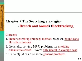
3. The branch-and-bound strategy • This strategy can be used to solve optimization problems without an exhaustive search in the average case.

4. Branch-and-bound strategy • 2 mechanisms: • A mechanism to generate branches when searching the solution space • A mechanism to generate bounds so that many braches can be terminated

5. Branch-and-bound strategy • It is efficient in the average case because many branches can be terminated very early. • Although it is usually very efficient, a very large search tree may be generated in the worst case. • Many NP-hard problems can be solved by B&B efficiently in the average case; however, the worst case time complexity is still exponential.

6. A Multi-Stage Graph Searching Problem. Find the shortest path from V0 to V3

7. E.G.:A Multi-Stage Graph Searching Problem

8. Solved by branch-and-bound (hill-climbing with bounds) A feasible solution is found whose cost is equal to 5. An upper bound of the optimal solution is first found here.

9. For Minimization Problems • Usually, LB<UB. • If LBUB, the expanding node can be terminated.  Upper Bound(for feasible solutions) Optimal Lower Bound(for expanding nods) 0

10. For Maximization Problems • Usually, LB<UB. • If LBUB, the expanding node can be terminated.  Upper Bound(for expanding nods) Optimal Lower Bound(for feasible solutions) 0

11. The traveling salesperson optimization problem • Given a graph, the TSP Optimization problem is to find a tour, starting from any vertex, visiting every other vertex and returning to the starting vertex, with the minimum cost. • It is NP-hard. • We try to avoid n! exhaustive search by the branch-and-bound technique on the average case. (Recall that O(n!)>O(2n).)

12. j i 1 2 3 4 5 6 7 1 ∞ 3 93 13 33 9 57 2 4 ∞ 77 42 21 16 34 3 45 17 ∞ 36 16 28 25 4 39 90 80 ∞ 56 7 91 5 28 46 88 33 ∞ 25 57 6 3 88 18 46 92 ∞ 7 7 44 26 33 27 84 39 ∞ The traveling salesperson optimization problem • E.g. A Cost Matrix for a Traveling Salesperson Problem.

13. The basic idea • There is a way to split the solution space (branch). • There is a way to predict a lower bound for a class of solutions. There is also a way to find an upper bound of an optimal solution. If the lower bound of a solution exceeds the upper bound, this solution cannot be optimal and thus we should terminate the branching associated with this solution.

14. Splitting • We split a solution into two groups: • One group including a particular arc • The other excluding the arc • Each splitting incurs a lower bound and we shall traverse the searching tree with the “lower” lower bound.

15. j i 1 2 3 4 5 6 7 1 ∞ 3 93 13 33 9 57 2 4 ∞ 77 42 21 16 34 3 45 17 ∞ 36 16 28 25 4 39 90 80 ∞ 56 7 91 5 28 46 88 33 ∞ 25 57 6 3 88 18 46 92 ∞ 7 7 44 26 33 27 84 39 ∞ The traveling salesperson optimization problem • The Cost Matrix for a Traveling Salesperson Problem. Step 1 to reduce: Search each row for the smallest value to j from i

16. j i 1 2 3 4 5 6 7 1 ∞ 0 90 10 30 6 54 (-3) 2 0 ∞ 73 38 17 12 30 (-4) 3 29 1 ∞ 20 0 12 9 (-16) 4 32 83 73 ∞ 49 0 84 (-7) 5 3 21 63 8 ∞ 0 32 (-25) 6 0 85 15 43 89 ∞ 4 (-3) 7 18 0 7 1 58 13 ∞ (-26) reduced:84 Step 2 to reduce: Search each column for the smallest value The traveling salesperson optimization problem • Reduced cost matrix: A Reduced Cost Matrix.

17. j i 1 2 3 4 5 6 7 1 ∞ 0 83 9 30 6 50 2 0 ∞ 66 37 17 12 26 3 29 1 ∞ 19 0 12 5 4 32 83 66 ∞ 49 0 80 5 3 21 56 7 ∞ 0 28 6 0 85 8 42 89 ∞ 0 7 18 0 0 0 58 13 ∞ (-7) (-1) (-4) The traveling salesperson optimization problem Table 6-5 Another Reduced Cost Matrix.

18. Lower bound • The total cost of 84+12=96 is subtracted. Thus, we know the lower bound of feasible solutions to this TSP problem is 96.

19. The traveling salesperson optimization problem • Total cost reduced: 84+7+1+4 = 96 (lower bound) decision tree: The Highest Level of a Decision Tree. • If we use arc 3-5 to split, the difference on the lower bounds is 17+1 = 18.

20. Heuristic to select an arc to split the solution space • If an arc of cost 0 (x) is selected, then the lower bound is added by 0 (x) when the arc is included. • If an arc <i,j> is not included, then the cost of the second smallest value (y) in row i and the second smallest value (z) in column j is added to the lower bound. • Select the arc with the largest (y+z)-x

21. j i 1 2 3 4 5 6 7 1 ∞ 0 83 9 30 6 50 2 0 ∞ 66 37 17 12 26 3 29 1 ∞ 19 0 12 5 ∞ 4 32 83 66 ∞ 49 80 5 3 21 56 7 ∞ 0 28 6 0 85 8 42 89 ∞ 0 7 18 0 0 0 58 13 ∞ For the right subtree (Arc 4-6 is excluded) We only have to set c4-6 to be . (-32) (-0) Total cost reduced: 96+32+0 = 128 (new lower bound) 21

22. For the left subtree (Arc 4-6 is included) • A Reduced Cost Matrix if Arc 4-6 is included. • 4th row is deleted. • 6th column is deleted. • We must set c6-4 to be . (The reason will be clear later.)

23. Loop Prevention • If arc i-j is to be added, then arc j-i must be excluded to prevent an unfeasible loop (by assigning the cost of j-i to be ). • If paths i1-i2-…-im and j1-j2-…-jn have already been included and a path from im to j1 is to be added, then the path from jn to j1 must be excluded (by assigning the cost of jn to i1 to be ).

24. Loop Preventing • For example, if 4-6, 2-1 are included and 1-4 is to be added, we must prevent 6-2 from being used by setting the cost of 6-2=. X

25. j i 1 2 3 4 5 7 1 ∞ 0 83 9 30 50 2 0 ∞ 66 37 17 26 3 29 1 ∞ 19 0 5 5 0 18 53 4 ∞ 25 (-3) 6 0 85 8 ∞ 89 0 7 18 0 0 0 58 ∞ For the left subtree(Arc 4-6 is included) • The cost matrix for all solutions with arc 4-6: A Reduced Cost Matrix for that in Table 6-6. • Total cost reduced: 96+3 = 99 (new lower bound)

26. Upper bound • We follow the best-first search scheme and can obtain a feasible solution with cost C. • C serves as an upper bound of the optimal solution and many branches may be terminated if their lower bounds are equal to or larger than C.

27. Fig 6-26 A Branch-and-Bound Solution of a Traveling Salesperson Problem.

28. The 0/1 knapsack problem • Positive integer P1, P2, …, Pn (profit) W1, W2, …, Wn (weight) M (capacity)

29. The 0/1 knapsack problem Fig. 6-27 The Branching Mechanism in the Branch-and-Bound Strategy to Solve 0/1 Knapsack Problem.

30. How to find the upper bound? • Ans: by quickly finding a feasible solution in a greedy manner: starting from the smallest available i, scanning towards the largest i’s until M is exceeded. The upper bound can be calculated.

31. i 1 2 3 4 5 6 Pi 6 10 4 5 6 4 Wi 10 19 8 10 12 8 (Pi/Wi Pi+1/Wi+1) The 0/1 knapsack problem • E.g. n = 6, M = 34 • A feasible solution: X1 = 1, X2 = 1, X3 = 0, X4 = 0, X5 = 0, X6 = 0 -(P1+P2) = -16 (upper bound) Any solution higher than -16 can not be an optimal solution.

32. How to find the lower bound? • Ans: by relaxing our restriction from Xi = 0 or 1 to 0  Xi 1 (knapsack problem)

33. The knapsack problem • We can use the greedy method to find an optimal solution for knapsack problem. • For example, for the state of X1=1 and X2=1, we have X1 = 1, X2 =1, X3 = (34-6-10)/8=5/8, X4 = 0, X5 = 0, X6 =0 -(P1+P2+5/8P3) = -18.5 (lower bound) -18 is our lower bound. (We only consider integers, since the benefits of a 0/1 knapsack problem will be integers.)

34. How to expand the tree? • By the best-first search scheme • That is, by expanding the node with the best lower bound. If two nodes have the same lower bounds, expand the node with the lower upper bound.

35. 0/1 Knapsack Problem Solved by Branch-and-Bound Strategy

36. Node 2 is terminated because its lower bound is equal to the upper bound of node 14. • Nodes 16, 18 and others are terminated because the local lower bound is equal to the local upper bound. (lower bound  optimal solution  upper bound)

37. The A* algorithm • Used to solve optimization problems. • Using the best-first strategy. • If a feasible solution (goal node) is selected to expand, then it is optimal and we can stop. • Estimated cost function of a node n : f(n) f(n) = g(n) + h(n) g(n): cost from root to node n. h(n): estimated cost from node n to a goal node. h*(n): “real” cost from node n to a goal node. f*(n): “real” cost of node n h(n)  h*(n)  f(n) = g(n) + h(n)  g(n)+h*(n) = f*(n) …………. (1) Estimated further cost should never exceed the real further cost.

38. Reasoning • Let t be the selected goal node. We have f*(t)=f(t)+h(t)=f(t)+0=f(t)…..(2) • Assume that t is not the optimal node. There must exist one node, say s, that has been generated but not selected and that will lead to the optimal node. • Since we take the best first search strategy, we have f(t)f(s)……(3). • We have f*(t)=f(t)f(s)f*(s) by Eqs. (1), (2) and (3), which means that s is not the node leading to the optimal node. Contradiction occurs. • Therefore, t is the optimal node.

39. The A* algorithm • Stop when the selected node is also a goal node. It is optimal iff h(n)h*(n) • E.g.: To find a shortest path from node s to node t

40. The A* algorithm • Step 1.

41. The A* algorithm • Step 2. Expand A

42. The A* algorithm • Step 3. Expand C

43. The A* algorithm • Step 4. Expand D

44. The A* algorithm • Step 5. Expand B

45. The A* algorithm • Step 6. Expand F I is selected to expand. The A* algorithm stops,since I is a goal node.

46. The A* Algorithm • Can be considered as a special type of branch-and-bound algorithm. • When the first feasible solution is found, all nodes in the heap (priority queue) are terminated. • * stands for “real” • “A* algorithm” stands for “real good algorithm”

47. Q&A