Download
1 / 20
210 likes | 353 Views
PLATON TINIOS & ANTIGONE LYBERAKI University of Piraeus Panteion University GREECE GREECE. GENDER GAPS AND LIFETIME INEQUALITY:. AN EMPIRICAL ANALYSIS OF MICRO-DATA FROM EUROPE. IFA Conference, Prague May 2012. A new – lifetime - perspective on an old issue.

E N D
PLATON TINIOS & ANTIGONE LYBERAKI University of Piraeus Panteion University GREECE GREECE GENDER GAPS AND LIFETIME INEQUALITY: AN EMPIRICAL ANALYSIS OF MICRO-DATA FROM EUROPE IFA Conference, Prague May 2012
A new –lifetime -perspective on an oldissue • Attempt to examine empirical implications of a novel and innovative micro dataset on an old issue of importance for gender balance • The old issue: ‘the’ Gender gap • Systematic differences in life chances between men & women • Observed in many dimensions, across countries, domains etc. • The new data: SHARELIFE • SHARE {w1 (2004) w2 (2007)} – European interdisciplinary panel of people 50+ (comparable to HRS in US, ELSA in UK)) • SHARELIFE (2009) – Retrospective lifetime questions for SHARE sample: • Childhood, education, health, family, work, etc for entire life. • The new perspective • How are gender gaps generated and how do they solidify in older ages? • Cross-country, cross-cohort, various dimensions • Key (ultimate) motivation: Palliative role of welfare states?? • A tour d’ horizon - attempt to quantify effects of different dimensions • Clarify issues – See the ‘lie of the land’
Outline: Halfway there… • Gender gaps and the life time perspective • Conceptual discussion. • Derive alternative measures of the gender gap appropriate to older populations aged 50+ • Vector of starting deprivation into scalar index of starting position • Examine socioeconomic mobility patterns • Attempt to disaggregate gender gap by a means of a reduced form equation
What is the gender gap? • Gender gap is an achievement gap • women are underpaid, undervalued and overworked. • Gender inequities in own income – economic independence deficit • Why doesn’t wage gap lead to rise in demand? • In general gender gaps are shrinking over time • What does it depend on? • Observables (education etc) / discrimination • Oaxaca (1973) method attempts to decompose • But: occupational segregation complicates • Bergmann (1974) overcrowding depresses wages • In career terms – snowball effect of low participation, few hours, lower wages • Evidence of polarisation among women • Cumulative earning gap (Luxembourg Income Study) • Could solidify further once retire from the labour market • SHARELIFE should provide data to examine issues as well as a new perspective:. • E.g. interdisciplinary insights + effect of Welfare State.
Conceptual issues • GENDER GAPS: • Multidimensional. Prominence to remuneration • Here: Cumulative (over life) or end-state. • Research strategy: DETERMINANTS • Split into different stages of life: • Initial, education, work/family, pension, health, • Social protection as a palliative influence through the life course • ‘Worlds of welfare capitalism’ -- chart the heyday of the Welfare Staete • 1st approach: Examine total effect on end- result • OLS of variables on end state Gender gap. • ≅ Reduced form. • Gives overview of total significance, though not causal (yet) • Could examine each stage in turn as stages cumulate over the life course, (plus partial attempts at amelioration) • Approach adopted in FRB (initial and work/family). • Axel Börsch-Supan et al 2011. Ongoing work. • E.g. early health⇒ Education⇒ Work chances⇒ End-state
How to define an over-50 Gender gap? • Gender gap usually identified as difference in wages and/or earnings. • End-state to be examined relatively well-defined • In a sample of people 50+, situation is more nuanced: • Some have never worked • Depending on conditions some decades ago. • Earningsexist for those who work. • Pensions cumulate past differences and correct • depending on welfare state structure and parameters of the preceding periods • Selection between earnings/pensions endogenous • Depends on personal preferences and welfare state parameters. (retirement ages) • In household level micro-data: • Savings also cumulate – income from property, rents, business • Categories of income accrue to household. (some social assistance) • Equivalence scales force gender equality by definition!
Two alternative courses of action • Define hybrid‘Personal income’ • Personal Income= Personal Income from Pensions + Personal Income from Employment + Equivalent income from other household level income sources • Not so much an ‘earnings gap’ but a ‘disposition of resources gap’ • Wider than gender gap -- cumulative effect over time • In addition to earnings encompasses other disadvantages • Narrower than gender gap --intra-household sharing • Rich housewives still rich, if household is rich • Decomposeinto (a) participation gap (b) retirement gap (c) earnings gap for those working (d) pensions gap for pensioners/ retired. • Richer diagnosis – less easy to interpret. • Two discrete choices – two alternative earnings determinations • More complex as a description
Overview of empirical work presented • Examination of end-state gaps • Under the two alternative definitions • Social Mobility analysis • Derivation of initial state ‘deprivation index’ • From initial conditions to end-conditions. • Reduced form OLS equation explaining end-gap*** • (Equivalent to Oaxaca-type study) • Groups of variables • ‘Pure gender’ effect – dummy • Effect of initial conditions • Education, work/family, pension • Quantify effect of different groups using predicted values for country groups and cohorts • For average values • For the poorest 20%
1: Crude gender gaps in 2007/9:Personalincome, 50+ population • Gap= 1- (Average for women/ Average for men) • Highest in South; smaller in North/Transition • Median gap – indication significant difference in distribution by gender • Gender gap widest in group 65-80. 80+ falls (influence of widows’ pensions)
Personal Income distribution by gender:Two extremes GR, SE) Gini M=0.437 F=0.574 High prevalence of zero incomes -- non-declaration? Non-working spouse in employee or pensioner household? Gini M=0.330 F=0.342
Detailed participation and separate earnings and pension gaps Participation gap Earnings and pensions gap (for those with +ve values)
Comparison of more familiar concepts: earnings and pension gaps • Define for two groups relatively close in age. • Earnings 50-64 • Pensions 65-80 • Could also be seen as ‘a look into the future of the pension gap’. • No clear pattern • Earnings>Pensions • DK, BE,CH,AT,CZ, ES • Pensions> Earnings • FR,IT,GR, PL • Almost the same • SE,DE • Need to understand differences
2. Mobility analysis • Childhood deprivation index • Described in Lyberaki, Tinios, Georgiadis 2011 • Related to end-state persistent poverty + soc. protection • Index of relative deprivation by country at age 10. • Weight more deprivation of those qualities more widely enjoyed • Constructed by 11 indicators (housing, family indicators) • Gives an idea of starting point • As chiefly family deprivation - gender balanced. • Cohort sensitive; though • However, the two sexes have different chances to alter personal position • Chart personal changes in rank • Change of quintile in distribution • Spearman rank order coefficients
Mobility – Change in quintile ranks Considerable change over time From starting point of gender equality (household status same for brother & sister) To end point Males move up Females down Biggest difference in South Spearman rank-order coefficient (on percentiles) Biggest difference in Continent Smallest in North
3. Description of Reduced form OLS equation • Dependent: Log (Personal income in 2007/9) • ‘Pure gender effect’ = Gender dummy • ‘Indirect gender effect’ = through gender differences in other determinants of income • (Assuming as 1st approx. coefficients same for men and women). • Initial effects – Cohort, Index, + GNP pc at 1960. • Education – years of schooling, higher dummy • Family status – Never married, widowed, divorced, married, Number of children • Work – years, years squared • Health – bad health during life, at end • Pensions - pensioner, years since pension • Country group dummies. Log of GDP pc in 1970 Approach similar to Oaxaca decomposition - proceed step by step
Pooled equation Pooled equation – presumes independent variables operate in the same way for men and women. Use as first approximation Reasonable fit Intuitive results “pure gender effect” – implies a gap of 33% if all else is equal. Employment crucial. All stages appear to have to ‘expected’ effect Country dummies included in lieu of social protection. Effect not easy to interpret.
OLS equation by gender By gender– presumes variables operate differently for men and women. Obviously so. Higher explanatory power for women. Initial conditions less important Education more Employment crucial (non-linear for W) Some variables have opposite sign M/F. (family variables) Some evidence of dampening by group – women benefit more from initial high GDP.
First results at decomposing differences • Use common Loading factors (pooled equation) i.e. no separate effect, (as in Neumark (1988) – non discrimination). How different are explanatory variables vs ‘pure’ gender effect (gender dummy) • Look at effect of different ‘endowments’ in four country groups. • Leave different loading factors for future (> complex interpretation) as in usual Oaxaca models. • Results considerably different by country group and cohort. • Most equalising effect in Nordics
Separate equations for work and pensions: preliminary observations In the earnings equation: • Family variables are very significant but of opposite sign by gender. • Favourable initial conditions affect men more than women • Wider differences M/W in effect of initial conditions • Years in employment has no apparent influence. Education has a very strong influence. • Being in a rich country affects men more than women • Collecting a pension depresses income from earnings In the pensions equation: • Overall gender effects are comparable to earnings. • Women have systematically lower pensions than men in the Continental countries (social insurance systems?). In Transition countries (ceteris paribus) women are better off. • Education is far more important for women (due to participation effects?). • Number of children exerts a strong negative effect on women – presumably accounting for dropping out of the labour market and other constraints on working. • Early deprivation has smaller effect, confined to men. It appears that the social protection system to some extent corrects for initial disadvantage. • Years of employment have a non-linear effect which diminishes with years • Early retirement is associated with lower pensions.
“There’s gold in them thar hills…”(Virginia gold rush – 1840s’) • First results are encouraging • Long way in a short space. Attempt to be parsimonious with numbers!! • There is much to be explained + much still left out. • Easy to lose the wood from the trees. • The wood: • The exercise using retrospective data of the European 50+ population may chart the success or failure of social protection system. • How are today’s pension gaps related to past events? What are the prospects for the future??