Download

1 / 24
240 likes | 560 Views
Binomial Distribution and Applications. Binomial Probability Distribution. A binomial random variable X is defined to the number of “successes†in n independent trials where the P(“successâ€) = p is constant. Notation: X ~ BIN(n,p)

E N D
Binomial Probability Distribution A binomial random variable X is defined to the number of “successes” in n independent trials where the P(“success”) = p is constant. Notation: X ~ BIN(n,p) In the definition above notice the following conditions need to be satisfied for a binomial experiment: • There is a fixed number of n trials carried out. • The outcome of a given trial is either a “success” or “failure”. • The probability of success (p) remains constant from trial to trial. • The trials are independent, the outcome of a trial is not affected by the outcome of any other trial.
Binomial Distribution • If X ~ BIN(n, p), then • where
Binomial Distribution • If X ~ BIN(n, p), then • E.g. when n = 3 and p = .50 there are 8 possible equally likely outcomes (e.g. flipping a coin) SSS SSF SFS FSS SFF FSF FFS FFF X=3 X=2 X=2 X=2 X=1 X=1 X=1 X=0 P(X=3)=1/8, P(X=2)=3/8, P(X=1)=3/8, P(X=0)=1/8 • Now let’s use binomial probability formula instead…
Binomial Distribution • If X ~ BIN(n, p), then • E.g. when n = 3, p = .50 find P(X = 2) SSF SFS FSS
Example: Treatment of Kidney Cancer • Suppose we have n = 40 patients who will be receiving an experimental therapy which is believed to be better than current treatments which historically have had a 5-year survival rate of 20%, i.e. the probability of 5-year survival isp = .20. • Thus the number of patients out of 40 in our study surviving at least 5 years has a binomial distribution, i.e. X ~ BIN(40,.20).
Results and “The Question” • Suppose that using the new treatment we find that 16 out of the 40 patients survive at least 5 years past diagnosis. • Q: Does this result suggest that the new therapy has a better 5-year survival rate than the current, i.e. is the probability that a patient survives at least 5 years greater than .20 or a 20% chance when treated using the new therapy?
What do we consider in answering the question of interest? We essentially ask ourselves the following: • If we assume that new therapy is no better than the current what is the probability we would see these results by chance variation alone? • More specifically what is the probability of seeing 16 or more successes out of 40 if the success rate of the new therapy is .20 or 20% as well?
Connection to Binomial • This is a binomial experiment situation…There are n = 40 patients and we are counting the number of patients that survive 5 or more years. The individual patient outcomes are independent and IF WE ASSUME the new method is NOT better then the probability of success is p = .20 or 20% for all patients. • So X = # of “successes” in the clinical trial is binomial with n = 40 and p = .20, i.e. X ~ BIN(40,.20)
Example: Treatment of Kidney Cancer • X ~ BIN(40,.20), find the probability that exactly 16 patients survive at least 5 years. • This requires some calculator gymnastics and some scratchwork! • Also, keep in mind we need to find the probability of having 16 or more patients surviving at least 5 yrs.
Example: Treatment of Kidney Cancer • So we actually need to find: P(X > 16) = P(X = 16) + P(X = 17) + … + P(X = 40) + … + = .002936 YIPES!
Enter n = sample sizex = observed # of “successes”p= probability of “success” Example: Treatment of Kidney Cancer • X ~ BIN(40,.20), find the probability that 16 or more patients survive at least 5 years. • USE COMPUTER! • Binomial Probability calculator in JMP probabilities are computed automatically for greater than or equal to and less than or equal to x.
Example: Treatment of Kidney Cancer • X ~ BIN(40,.20), find the probability that 16 or more patients survive at least 5 years. • USE COMPUTER! • Binomial Probability calculator in JMP P(X > 16) = .0029362 The chance that we would see 16 or more patients out of 40 surviving at least 5 years if the new method has the same chance of success as the current methods (20%) is VERY SMALL, .0029!!!!
Conclusion • Because it is high unlikely (p = .0029) that we would see this many successes in a group 40 patients if the new method had the same probability of success as the current method we have to make a choice, either … • we have obtained a very rare result by dumb luck. OR • our assumption about the success rate of the new method is wrong and in actuality the new method has a better than 20% 5-year survival rate making the observed result more plausible.
Sign Test • The sign test can be used in place of the paired t-test when we have evidence that the paired differences are NOT normally distributed. • It can be used when the response is ordinal. • Best used when the response is difficult to quantify and only improvement can be measured, i.e. subject got better, got worse, or no change. • Magnitude of the paired difference is lost when using this test.
Example: Sign Test • A study evaluated hepatic arterial infusion of floxuridine and cisplatin for the treatment of liver metastases of colorectral cancer. • Performance scores for 29 patients were recorded before and after infusion. • Is there evidence that patients had a better performance score after infusion?
Sign Test • The sign test looks at the number of (+) and (-) differences amongst the nonzero paired differences. • A preponderance of +’s or –’s can indicate that some type of change has occurred. • If in reality there is no change as a result of infusion we expect +’s and –’s to be equally likely to occur, i.e. P(+) = P(-) = .50 and the number of each observed follows a binomial distribution.
Example: Sign Test • Given these results do we have evidence that performance scores of patients generally improves following infusion? • Need to look at how likely the observed results are to be produced by chance variation alone.
18 nonzeros differences, 11 +’s 7 –’s Example: Sign Test - + + - + - - + + + + + + - - + - +
Example: Sign Test • If there is truly no change in performance as a result of infusion the number of +’s has a binomial distribution with n = 18 and p = P(+) = .50. • We have observed 11 +’s amongst the 18 non-zero performance differences. • How likely are we to see 11 or more +’s out 18? P(X > 11) = .2403 for a binomial n = 18, p = .50 • There is 24.03% chance we would see this many improvements by dumb luck alone, therefore we are not convinced that infusion leads to improvement (Remember less than .05 or a 5% chance is what we are looking for “statistical significance”)
Example 2: Sign Test Resting Energy Expenditure (REE) for Patient with Cystic Fibrosis • A researcher believes that patients with cystic fibrosis (CF) expend greater energy during resting than those without CF. To obtain a fair comparison she matches 13 patients with CF to 13 patients without CF on the basis of age, sex, height, and weight. She then measured there REE for each pair of subjects and compared the results.
Example 2: Sign Test There are 11 +’s & 2 –’s out of n = 13 paired differences.
Example 2: Sign Test The probability of seeing this many +’s is small. We conclude that when comparing individuals with cystic fibrosis to healthy individuals of the same gender and size that in general those with CF have larger resting energy expenditure (REE) (p = .0112).