Download
1 / 41
410 likes | 491 Views
V16 Stochastic processes in cells. 3 aspects of genetic circuits control dynamic cellular behaviors: - the circuit architecture or pattern of regulatory interactions among genetic elements - quantitative parameter values: parameter strengths ...

E N D
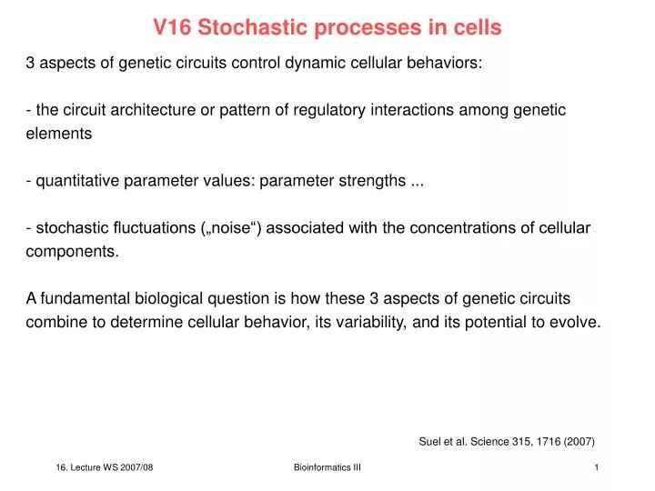
V16 Stochastic processes in cells 3 aspects of genetic circuits control dynamic cellular behaviors: - the circuit architecture or pattern of regulatory interactions among genetic elements - quantitative parameter values: parameter strengths ... - stochastic fluctuations („noise“) associated with the concentrations of cellular components. A fundamental biological question is how these 3 aspects of genetic circuits combine to determine cellular behavior, its variability, and its potential to evolve. Suel et al. Science 315, 1716 (2007) Bioinformatics III
Bacillus subtilis Competence in B. subtilis is a stress response. It allows cells to take up DNA from the environment. Differentiation into competence is transient. Suel et al. Science 315, 1716 (2007) Competence is a probabilistic and transient differentiation process regulated by a genetic circuit. Pinit: The rate of entering the competent state from the vegetative state comp: amount of time spent in the competent state The ComK transcription factor concentration is high (pink region) when cells are competent and low (green region) when they are growing vegetatively. Bioinformatics III
Bacillus subtilis The genetic basis for this behavior is a circuit involving comK and comS. The transcription factor ComK is necessary and sufficient for differentiation into competence. ComK positively autoregulates its own expression but is degraded by the ClpP-ClpC-MecA protease complex. ComS competitively inhibits this degradation and is repressed in competent cells, forming a negative feedback loop. Map of the core competence circuitry. Key features include positive transcriptional autoregulation of comK and a negative feedback loop in which ComK inhibits (possibly indirectly) expression of ComS, which in turn interferes with degradation of ComK. The graphs below the PcomK and PcomS promoters define parameters of this system: Expression rates change from K to K and from S to S respectively, as ComK concentration increases during competence. Suel et al. Science 315, 1716 (2007) Bioinformatics III
Bacillus subtilis k and s, the basal expression rates of comK and comS, are expected to affect the behavior of the circuit. To manipulate these parameters, an additional copy of either comS or comK under the control of an inducible promoter denoted Phyp generating the Hyper-k and Hyper-s, was inserted into one chromosome. K and S qualitatively change the dynamics of the competence circuit and independently tune the probability of initiation (Pinit) and mean duration (comp) of competence events. (A and B) Filmstrips and PcomG-cfp time traces (for individual cells) of competence events obtained in Hyper-K (Phypk-comK) and Hyper-S (Phyp-comS) strains at the IPTG concentrations and times (hours) indicated. PcomG-cfp and PcomS-yfp activities are depicted in red and green, respectively. Sporulating cells are seen in white. Cells that did not sporulate were prone to lysis toward the end of movie acquisition. Bioinformatics III
Bacillus subtilis K and S qualitatively change the dynamics of the competence circuit and independently tune the probability of initiation (Pinit) and mean duration (comp) of competence events. (A and B) Filmstrips and PcomG-cfp time traces (for individual cells) of competence events obtained in Hyper-K (Phypk-comK) and Hyper-S (Phyp-comS) strains at the IPTG concentrations and times (hours) indicated. PcomG-cfp and PcomS-yfp activities are depicted in red and green, respectively. Sporulating cells are seen in white. Cells that did not sporulate were prone to lysis toward the end of movie acquisition. Bioinformatics III
Simulation model To better understand independent tuning of Pinit and comp, as well as reliable maintenance of excitability, use 2 simulation models of the core interactions in the competence regulation circuitry. - 2 continuous ODEs for the concentrations of comK and comS - stochastic simulations that account for intrinsic noise of biochemical reactions. Aim: analyze the continuous model to determine parameter dependence and to identify a biologically reasonable parameter regime in which the discrete model produced results consistent with experiments. The continuous model is required to remain in the excitable regime as the S value was varied by a factor of 6 and the stochastic counterpart is required to generate the observed independent tunability of Pinit and comp. parameter set that accounts for both maintenance of excitability at high S and independent tunability by S and K. Bioinformatics III
Core compentence circuit K : concentration of ComK S: concentration of ComS rearrange into Suel et al. Science 315, 1716 (2007) Bioinformatics III
Phase diagram of continuous model Bioinformatics III
Phase diagram of continuous model Bioinformatics III
V16 Stochastic processes in cells Bioinformatics III
Stochastic model Bioinformatics III
Stochastic model Bioinformatics III
strong effect of K on Pinit Within the model, increasing K increased the probability that vegetative cells reach the minimum concentration of ComK necessary to initiate competence, explaining the strong effect of K on Pinit. Bioinformatics III
Effect of ComS expression Bioinformatics III
V16 Stochastic processes in cells Bioinformatics III
Can one make comp more precise? To explore the effects of perturbing the circuit architecture, we reengineered the competence circuit using Rok, a protein that binds to PcomK and represses its expression. We inserted a copy of rok under the control of PcomG, creating an additional negative feedback loop onto comK (Fig. 3A). Bioinformatics III
What determines Pinit? Here, use a mutant that grows very long cells variations of the concentrations become smaller. D: the onset probability Pinit is clearly reduced. Control experiments: the expression level of 2 other genes is unchanged Bioinformatics III
Conclusions Noise may play at least three different functional roles in competence. First, noise could be responsible for the observed variability in duration. Second, noise may be necessary to maintain excitability over a wide parameter range, by inducing escape from states of high ComK concentration. Third, noise appears to have a pivotal role in competence initiation and thus should be considered alongside genetic parameters and circuit architecture to comprehensively understand differentiation at the single cell level. Quantitative analysis of a genetic system beyond its normal operating regime, including gene expression strengths, circuit architecture, and noise levels, strongly constrains dynamical models. The competence regulation system maintains excitable behavior over a broad range of parameter values. Experimentally, K and S enable Pinit and tcomp to be tuned independently, allowing the system, in theory, to adapt to independent selective pressures during evolution. The circuit can also access different dynamic regimes, such as oscillation and bistability, indicating its potential to evolve alternative qualitative behaviors. Bioinformatics III
New challenge: Electron Tomography Method overview a) The electron beam of an EM microscope is scattered by the central object and the scattered electrons are detected on the black plate. By tilting the object in small steps, collect electrons scattered at different angles. b) reconstruction in the computer. Back-projection (Fourier method) of the scatter-information at different angles. The superposition generates a three-dimensional tomogrom. Sali et al. Nature 422, 216 (2003) Bioinformatics III
Identification of macromolecular complexes in cryoelectron tomograms of phantom cells Idea: construct model system with well-defined properties. Prepare „phantom cells“ (ca. 400 nm diameter) with well-defined contents: liposomes filled with thermosomes and 20S proteasomes. Thermosome: 933 kD, 16 nm diameter, 15 nm height, subunits assemble into toroidal structure with 8-fold symmetry. 20S proteasome: 721 kD, 11.5 nm diameter, 15 nm height, subunits assemble into toroidal structure with 7-fold symmetry. Collect Cryo-EM pictures of phantom cells for a tilt series from -70º until +70º with 1.5º increments. Aim: identify and map the 2 types of proteins in the phantom cell. This is a problem of matching a template, ideally derived from a high-resolution structure, to an image feature, the target structure. Frangakis et al., PNAS 99, 14153 (2002) Bioinformatics III
Detection and idenfication strategy The correlation of two functions is defined as Correlation theorem for the transform pairs: Frangakis et al., PNAS 99, 14153 (2002) Bioinformatics III
Search strategy • Adjust pixel size of templates to the pixel size of the EM 3D reconstruction. • The gray value of a voxel (volume element) containing ca. 30 atoms is obtained by summation of the atomic number of all atoms positioned in it. • Possible search strategies: • Scan reconstructed volume by using small boxes of the size of the target structure (real space method) • Paste template into a box of the size of the reconstructed volume (Fourier space method). This method is much more efficient. Frangakis et al., PNAS 99, 14153 (2002) Bioinformatics III
Correlation with Nonlinear Weighting The correlation coefficient CC is a measure of similarity of two features e.g. a signal x (image)and a template r both with the same size R. Expressed in one dimension: are the mean values of the subimage and the template. The denominators are the variances To derive the local-normalized cross correlation function or, equivalently, the correlation coefficients in a defined region R around each voxel k, which belongs to a large volume N (whereby N >> R), nonlinear filtering has to be applied. This filtering is done in the form of nonlinear weighting. Frangakis et al., PNAS 99, 14153 (2002) Bioinformatics III
Raw data • Central x-y slices through the 3D reconstructions of ice-embedded phantom cells filled with • 20S proteasomes, • thermosomes, • and a mixture of both particles. • At low magnification, the macromolecules appear as small dots. Frangakis et al., PNAS 99, 14153 (2002) Bioinformatics III
Correlation coefficients • Histogram of the correlation coefficients of the particles found in the proteasome-containing phantom cell scanned with the "correct" proteasome and the "false" thermosome template. Of the 104 detected particles, 100 were identified correctly. The most probable correlation coefficient is 0.21 for the proteasome template and 0.12 for the thermosome template. • Histogram of the correlation coefficients of the particles found in the thermosome-containing phantom cell. Of the 88 detected particles, 77 were identified correctly. The most probable correlation value is 0.21 for the thermosome template and 0.16 for the proteasome template. • Detection in (a) works well, but is somehow problematic in (b) because (correct) thermosome and proteasome are not well separated. Frangakis et al., PNAS 99, 14153 (2002) Bioinformatics III
Reconstruction of phantom cell Volume-rendered representation of a reconstructed ice-embedded phantom cell containing a mixture of thermosomes and 20S proteasomes. After applying the template-matching algorithm, the protein species were identified according to the maximal correlation coefficient. The molecules are represented by their averages; thermosomes are shown in blue, the 20S proteasomes in yellow. The phantom cell contained a 1:1 ratio of both proteins. The algorithm identifies 52% as thermosomes and 48% as 20S proteasomes. Frangakis et al., PNAS 99, 14153 (2002) Bioinformatics III
Electron tomography • Method has very high computational cost. • Observation: biological cells are not packed so densely as expected, • allowing the identification of single proteins and protein complexes • Problem for real cells: molecular crowding. • Potential difficulties to identify spots. • - need to increase spatial resolution of tomograms Frangakis et al., PNAS 99, 14153 (2002) Bioinformatics III
Reconstruction of endoplasmatic reticulum Picture rights shows rough endoplasmatic reticulum (membrane network in eukaryotic cells that generates proteins and new membranes) coated with ribosomes. The picture is taken from an intact cell. Membranes are shown in blue, the ribosomes in green-yellow. http://science.orf.at/science/news/61666 Dept. of Structural Biology, Martinsried Bioinformatics III
Reconstruction of the Golgi apparatus The Golgi complex is the organelle in which newly synthesized lipids and proteins are modified and targeted for distribution to various cellular and extracellular destinations. HVEM tomographic reconstruction of a portion of the Golgi ribbon from a fast frozen, freeze-substitution fixed NRK cell. Two serial 4-nm slices extracted from the tomogram are shown in a and b. Comparison of the images shows how little is changed from one such slice to its neighbor; e.g., the position of the microtubule (red arrow). (a) Membranes of individual Golgi and ER cisternae are clearly seen. (b) In analyzing the data, different cisternae were modeled by placing points along the membranes that delimit them, connecting the points with colored line segments, and building closed contours that model the different membrane compartments of a given slice. Ladinsky et al. J. Cell. Biol. 144, 1135 (1999) Bioinformatics III
Reconstruction of the Golgi apparatus c and d are renditions of the surfaces fit to all of the contours for each object modeled in this Golgi region. The model viewed in c is in the same orientation as the tomographic slices. d shows a cisside view with the cis ER removed to provide a better view of the ERGIC elements and the underlying Golgi cisternae. The 44 elements of the ERGIC are discontinuous, display no coated budding profiles, and do not appear to be flattened against the cis-most cisterna. Free vesicles in wells and the NCR (white) have unrestricted access to the cis side of the stack. The colors used to represent different components of the model are the same in all figures: ER, bluegray; ribosomes, small purple spheres; ERGIC, yellow; Golgi cisterna: C1, green; C2, purple; C3, rose; C4, olive; C5, pink; C6, bronze; C7, red. Polymorphic structures in the NCR are light pink and gold. Non–clathrincoated budding profiles on cisternae C1–C6, blue stippling. Clathrin-coated buds on C7, yellow stippling. Bars, 250 nm. Ladinsky et al. J. Cell. Biol. 144, 1135 (1999) Bioinformatics III
Reconstruction of the Golgi apparatus Ladinsky et al. J. Cell. Biol. 144, 1135 (1999) Bioinformatics III
Mitochondria Surface-rendered representation of the mitochondrial reconstruction in two different orientations. The crista membrane that forms a three-dimensional network of interconnected lamellae is continuous with the inner boundary membrane (both shown in yellow). The outer membrane (magenta) is separated from the inner boundary membrane by a narrow intermembrane space of remarkably constant width. Nicastro et al. J. Struct. Biol. 129, 48 (2000) Bioinformatics III
The nuclear pore complex Nuclear pore complexes (NPCs) mediate the exchange of macromolecules between the nucleus and the cytoplasm. These large assemblies (ca. 120 megadaltons in metazoa) are constructed from about 30 different proteins, the nucleoporins. (E) Surfacerendered representation of a segment of nuclear envelope (NPCs in blue, membranes in yellow). The dimensions of the rendered volume are 1680 nm 984 nm 558 nm. The number of NPCs was ca. 45/m2. Beck et al. Science 306, 1387 (2004) Bioinformatics III
The nuclear pore complex Fig. 2. Structure of the Dictyostelium NPC. (A). Cytoplasmic face of the NPC in stereo view. The cytoplasmic filaments are arranged around the central channel; they are kinked and point toward the CP/T. (B) Nuclear face of the NPC in stereo view. The distal ring of the basket is connected to the nuclear ring by the nuclear filaments. (C) Cutaway view of the NPC with the CP/T removed. Beck et al. Science 306, 1387 (2004) Bioinformatics III
Herpes simplex virus Segmented surface rendering of a single virion tomogram after denoising. (A) Outer surface showing the distribution of glycoprotein spikes (yellow) protruding from the membrane (blue). (B) Cutaway view of the virion interior, showing the capsid (light blue) and the tegument “cap” (orange) inside the envelope (blue and yellow). pp, proximal pole; dp, distal pole. Scale bar, 100 nm. (C) Segmented surface rendering of a virion portion. Tegument is orange, membrane is blue, and spikes are yellow. Scale bars, 20nm. Grünewald et al. Science 302, 1396 (2003) Bioinformatics III
3D reconstruction of Saccharomyces cerevisae cell Larabell et al. Mol. Biol. Cell 15, 957 (2004) Bioinformatics III
3D reconstruction of Saccharomyces cerevisae cell Larabell et al. Mol. Biol. Cell 15, 957 (2004) Bioinformatics III
a nerve cell Tomographic reconstruction of neuronal spiny dendrite from the rat neostriatum (C) A surface reconstruction of the segmented volume showing the dendritic shaft in blue and the dendritic spines in red. (E) Segmented reconstruction of the node showing the major components in different colors. Yellow, compact myelin; red, axolemma; blue, paranodal loops; white, mitochondria; green, intraaxonal vesicles. Martone et al. J. Struct. Biol. 138, 145 (2002) Bioinformatics III
Reconstruction of actin filaments Actin filaments are structural proteins – they form filaments which span the entire cell. They stabilize the cellular shape, are required for motion, and are involved in important cellular transport processes (molecular motors like kinesin walk along these filaments). Shown is the cytoskeleton of Dictyostelium. Apparently, filaments cross and bridge each other at different angles, and are connected to the cell membrane (right picture). Actin filaments are shown in brown. The cell segment left has a size of 815 x 870 x 97 nm3. Middle: single actin filaments connected at different angles. Right: actin filaments (brown) binding to the cell membrane (blue). http://science.orf.at/science/news/61666 Dept. of Structural Biology, Martinsried Bioinformatics III
Science fiction • Reconstruct proteome of real biological cells. • Required steps: • obtain EM maps of isolated (e.g. 6000 yeast) proteins • enhance resolution of tomography • speed up detection algorithm http://science.orf.at/science/news/61666 Dept. of Structural Biology, Martinsried Bioinformatics III
Summary • The structural characterization of large multi-protein complexes and the resolution of cellular architectures will likely be achieved by a combination of different methods in structural biology: • X-ray crystallography and NMR for high-resolution structures of single proteins and pieces of protein complexes • (Cryo) Electron Microscopy to determine medium-resolution structures of entire protein complexes • Stained EM for still pictures at medium-resolution of cellular organells • (Cryo) Electron Tomography for 3-dimensional reconstructions of biological cells and for identification of the individual components. • Mapping and idenfication steps require heavy computation. • Employ protein-protein docking as a help to identify complexes? • teams of experimentalists and bioinformaticians • - Sali & Baumeister, Sali & Chu • - Russell & Böttcher • - Wriggers & J. Frank, M. Radermacher & J. Frank Bioinformatics III