15. Ultrafast Laser Spectroscopy

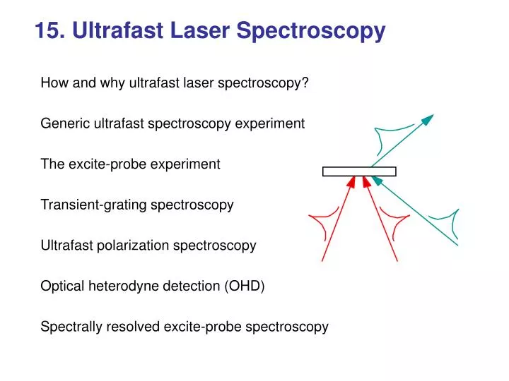
1. 15. Ultrafast Laser Spectroscopy How and why ultrafast laser spectroscopy? Generic ultrafast spectroscopy experiment The excite-probe experiment Transient-grating spectroscopy Ultrafast polarization spectroscopy Optical heterodyne detection (OHD) Spectrally resolved excite-probe spectroscopy

2. Ultrafast Laser Spectroscopy: Why? Most events that occur in atoms and molecules occur on fs and ps time scales. The length scales are very small, so very little time is required for the relevant motion. Fluorescence occurs on a ns time scale, but competing non-radiative processes only speed things up because relaxation rates add: 1/tex = 1/tfl + 1/tnr Biologically important processes utilize excitation energy for purposes other than fluorescence and hence must be very fast. Collisions in room-temperature liquids occur on a few-fs time scale, so nearly all processes in liquids are ultrafast. Semiconductor processes of technological interest are necessarily ultrafast or we wouldn’t be interested.

3. “Signal pulse” Medium under study Signal pulse energy Variably delayed “Probe pulse” Delay “Excitation pulses” Ultrafast laser spectroscopy involves studying ultrafast events that take place in a medium using ultrashort pulses and delays for time resolution. It usually involves exciting the medium with one (or more) ultrashort laser pulse(s) and probing it a variable delay later with another. Ultrafast Laser Spectroscopy: How? The signal pulse energy (or change in energy) is plotted vs. delay. The experimental temporal resolution is the pulse length.

4. What’s going on in spectroscopy measurements? Unexcited medium Excited medium Unexcited medium absorbs heavily at wavelengths corresponding to transitions from ground state. Excited medium absorbs weakly at wavelengths corresponding to transitions from ground state. The excite pulse(s) excite(s) molecules into excited states. Because there are now fewer molecules in the ground state to absorb the probe pulse, this decreases the medium’s absorption coefficient. The excited states only live for a finite time (this is the quantity we’d like to find!), so the absorption recovers. And the refractive index changes (and recovers), too.

5. The simplest ultrafast spectroscopy method is The Excite-Probe Technique. Change in probe pulse energy Delay This involves exciting the sample with one pulse, probing it with another a variable delay later, and measuring the change in the transmitted probe pulse average power vs. delay: The excite pulse changes the sample absorption seen by the probe pulse. Excite pulse Slow detector Sample Probe pulse Lens Delay The excite and probe pulses can be different colors. This technique is also called the “Pump-Probe” Technique.

6. Lock-in Detection greatly increases the sensitivity in excite-probe experiments. This involves chopping the excite pulse at a given frequency and detecting at that frequency with a lock-in detector: The excite pulse periodically changes the sample absorption seen by the probe pulse. Chopper Chopped excite pulse train Slow detector Lock-in detector Sample Lens The lock-in detects only one frequency component of the detector voltage—chosen to be that of the chopper. Probe pulse train Delay Lock-in detection automatically subtracts off the transmitted power in the absence of the excite pulse. With high-rep-rate lasers, it increases sensitivity by several orders of magnitude!

7. Modeling excite-probe measurements Let the unexcited medium have an absorption coefficient, a0. Immediately after excitation, the absorption decreases by Da0. Since the excited states usually decay exponentially: Da(t) = Da0exp(–t /tex) for t > 0 where t is the delay after excitation, and tex is the excited state lifetime. So the transmitted probe-beam intensity—and hence pulse energy and average power—will depend on the delay, t, and the lifetime, tex: Itransmitted(t) = Iincidentexp{–[a0 – Da0exp(–t /tex)]L} where L= sample length = Iincidentexp{–a0L} exp{Da0exp(–t /tex)L} [ Iincidentexp{–a0L}] {1+Da0exp(–t /tex)L} assuming Da0 L << 1 Itransmitted(-) {1+Da0exp(–t /tex)L}

8. Modeling excite-probe measurements (cont’d) Excite transition Probe transition The relative change in transmitted intensity vs. delay, t, is: Change in probe-beam intensity DT(t) /T = = [Itransmitted(t) –Itransmitted()] /Itransmitted() Da0 exp(–t /tex)L} Delay, t 0 More complex decays can be seen if intermediate states are populated or if the motion is complex. Imagine probing an intermediate transition, whose states temporarily fill with molecules on their way back down to the ground state: Excited molecules in state 2: stimulated emission of probe 3 2 Change in probe-beam transmitted intensity Excited molecules in state 1: absorption of probe 0 1 Delay, t 0 0

9. Excite-probe measurements in DNA DNA bases undergo photo-oxidative damage, which can yield mutations. Understanding the photo-physics of these important molecules may help to understand this process. Pecourt, et al., Ultrafast Phenomena XII, p.566 (2000).

10. Excite-probe measurements of bacteriorhodopsin Rhodopsin is the main molecule involved in vision. After absorbing a photon, rhodopsin undergoes a many-step process, whose first three steps occur on fs or ps time scales and are poorly understood. Native Artificial Probe at 460 nm (increased absorption): Zhong, et al., Ultrafast Phenomena X, p. 355 (1996). Probe at 860 nm (stimulated emission): Excitation populates a new state, which absorbs at 460 nm and emits at 860 nm. It was thought that this state involved motion of the carbon atoms (12, 13, 14). But an artificial version rhodopsin, with those atoms held in place, also reveals this change and does so even faster.

11. Excite-probe measurements of Hypericin, an anti-viral substance When excited by light, Hypericin deactivates HIV. So it’s important to understand its behavior. These curves (for two different solvents) show the rise time for a proton-transfer process important in its biological activity. Relative change in absorbance M.J. Fehr, et al., Ultrafast Phenomena IX, pg. 462 (1994).

12. Excite-probe measurements of Terawatt femtosecond UV pulses in water High-intensity UV ultrashort pulses may someday be used in surgery. So understanding what these pulses do to water is important. Hydrated electrons are formed in very high concentrations (0.01 molar). The induced absorption seen here is very high! Pommeret, et al., Ultrafast Phenomena XII, p. 536 (2000).

13. Excite-Probe Reflection Spectroscopy Exciting a surface and probing its reflectivity later reveals surface physics. Here, a quantum wire is studied using ultrashort pulses in a near-field scanning optical micro-scope to yield 200-nm spatial resolution, too! Emiliani, et al., Ultrafast Phenomena XII, p. 256 (2000).

14. Excite-probe measurements can reveal quantum beats: Theory Excitation-pulse spectrum 2 1 Probe pulse Excite pulse 0 Since ultrashort pulses have broad bandwidths, they can excite two or more nearby states simultaneously. Probing the 1-2 superposition of states can yield quantum beats in the excite-probe data.

15. Excite-probe measurements can reveal quantum beats: Experiment Here, two nearby vibrational states in molecular iodine interfere. These beats also indicate the motion of the molecular wave packet on its potential surface. A small fraction of the I2 molecules dissociate every period. Zadoyan, et al., Ultrafast Phenomena X, p. 194 (1996).

16. Quantum Beats in Polymers Using 5-fs Pulses Excite-probe measurements in polydiacetylene show several different frequencies, implying several (vibrational) states were excited. Kobayashi, Ultrafast Phenomena XII, p. 575 (2000).

17. The Coherence Spike in Ultrafast Spectroscopy Excite pulse Sample Probe pulse When the delay is zero,other nonlinear-optical processes occur, a involving coherent 4WM between the beams,and generatingaadditional signal that is not described by the simple Da model. As in autocorrelation, it’s called the “coherence spike” or “coherent artifact.” Sometimes you see it; sometimes you don’t. This spike could be a very very fast event that couldn’t be resolved. Or it could be a coherence spike. Intensity fringes in sample when pulses arrive simultaneously When the two input pulses arrive simultaneously, they also induce a grating, which diffracts light from each beam into the other.

18. A background-free ultrafast spectroscopy method is The Transient-Grating Technique. This involves exciting the sample with two simultaneous excitation pulses, inducing a weak diffraction grating, probing it with another pulse a variable delay later, and measuring the diffracted pulse average power vs. delay: Intensity fringes in sample due to excitation pulses Excite pulse #1 Sample Excite pulse #2 Slow detector Diffracted pulse Probe pulse Delay The excite pulses have a spatially sinusoidal energy deposition in the sample. The sample absorption and refractive index will now vary sinusoidally in space. These “induced gratings” (in amplitude and phase) will diffract a probe pulse while the excitation exists. Diffracted pulse energy Delay, t 0

19. A transient-grating measurement may still have a coherence spike! Diffracted beam intensity Delay, t 0 When all the pulses overlap in time, who’s to say which are the excitation pulses and which is the probe pulse? Intensity fringes in sample due to an excitation pulse and the probe acting as an excitation pulse Excite pulse #1 (acting as the probe) Excite pulse #2 Probe pulse (acting as an excite pulse) Delay A transient-grating experiment with a coherence spike:

20. What the Transient-Grating Technique measures Diffracted beam intensity Transmitted intensity Delay, t 0 The Transient Grating (TG) technique measures the Pythagorean sum of the changes in the absorption and refractive index. The diffraction efficiency, , is given by: Absorption (amplitude) grating Refractive index (phase) grating This is in contrast to the excite-probe technique, which is only sensitive to the change in absorption and depends on it linearly. If the absorption grating dominates and the excite-probe decay is exp(-ex), then the TG decay will be exp(-2ex): H. Eichler, Laser-Induced Dynamic Gratings, Springer-Verlag, 1986.

21. Transient Orientation Gratings You might think that a grating can be induced only by a sinusoidal intensity pattern (caused by the interference of two parallel-polarized beams). But orthogonally polarized beams, which have a constant intensity vs. position, also induce a grating! An “orientation grating.” Variation of the electric field vs. position: Orientation gratings can also decay due to orientational relaxation.

22. Induced gratings can also decay by diffusion. Diffusion can wash out an induced grating. Sometimes diffusion is faster than excited-state decay. t = 0 L Excited-state density t >> 0 Position (x) Diffusion occurs on a time scale that depends on the grating fringe spacing. If the fringes are closely spaced, diffusion is very fast; if the fringes are far apart, then it’s much slower. Varying the grating fringe spacing can determine the time scales for both decay mechanisms. where D = diffusion coeff

23. Transient-Grating Measurements in Multiple Quantum Wells Both concentration (amplitude) and orientation (spin) gratings induced by excite beams with parallel and perpendicular polarizations. The orientation grating decays much faster. Note the variation in decay time for different fringe spacings, illustrating the role of diffusion. Cameron, et al., Ultrafast Phenomena X, p. 408 (1996).

24. Time-Resolved Fluorescence is also useful. Excite pulse Fluorescence SFG crystal Slow detector Sample Probe pulse Lens Fluorescent beam power Delay Delay Exciting a sample with an ultrashort pulse and then observing the fluoresccence vs. time also yields sample dynamics. This can be done by directly observing the fluroescence or, if it’s too fast, by time-gating it with a probe pulse in a SFG crystal:

25. Time-Resolved Fluorescence Decay When different tissues look alike (i.e., have similar absorption spectra), looking at the time-resolved fluorescence can help distinguish them. Here, a malignant tumor can be distinguished from normal tissue due to its longer decay time. Svanberg, Ultrafast Phenomena IX, p. 34 (1994).

26. Ultrafast Polarization Spectroscopy 45˚ polarized excite pulse 90˚ polarizer Sample HWP Probe pulse 0˚ polarizer Delay A 45˚-polarized excite pulse will induce birefringence in an ordinarily isotropic sample. A variably delayed probe pulse between crossed polarizers can watch the birefringence decay, revealing the sample orientational relaxation. Light changing the refractive index of a medium is called the “Kerr effect.” It’s also possible to change the absorption coefficient differently for the two polarizations. This is called an “induced dichroism.” It also rotates the probe polarization and can also be used to study orientational relaxation.

27. Nice Features of Ultrafast Polarization Spectroscopy It’s as easy to set up as excite-probe (just cross two beams in space and time). It’s almost background-free (crossed polarizers transmit as little as 10-6 of the incident light). Unlike excite-probe, it measures both absorption and phase effects. It can use lock-in detection. And simultaneously, it can use “optical heterodyne detection,” which optimizes the signal-to-noise ratio.

28. Heterodyned Ultrafast Polarization Spectroscopy 45˚ polarized excite pulse 90˚ polarizer Sample HWP Probe pulse Set up is exactly the same, except for this polarizer! 1˚ polarizer Delay “Optical Heterodyne Detection” (OHD) polarization spectroscopy involves slightly uncrossing the polarizers. This allows some of the probe pulse to leak into the detector and combine coherently with the signal pulse. This trivial (seemingly inappropriate!) change can actually improve the sensitivity by many orders of magnitude!

29. Heterodyned Ultrafast Polarization Spectroscopy Heterodyned polarization spectroscopy adds a small amount of the probe pulse, dEprobe(t), to the (even smaller) signal pulse. As a result, we now detect the squared magnitude of the sum of these two fields: As long as the leaked probe intensity >> the signal intensity, we can neglect the latter: This yields a signal term proportional to Esig(t), which is much larger than its squared magnitude. And it also yields its phase. As long as the probe intensity is stable, this yields a huge improvement in sensitivity.

30. Heterodyned Ultrafast Polarization Spectroscopy of Liquids 2 Using different colors for the excite and probe pulses, this technique is called the Optical Heterodyne Detection-Raman-Induced Kerr Effect Spectroscopy (OHD-RIKES). Probe pulse wpr Excite pulse wex 1 w10 0 The excite pulse can induce a change in the refractive index seen by the probe pulse, which is enhanced when wex – wpr = w10 Sample media are various amides. Notice how very clean the data are. Castner and Chang, Ultrafast Phenomena X, p. 296 (1996).

31. Heterodyned Ultrafast Polarization Spectroscopy of CS2 OHD-RIKES study of CS2 at different temperatures. Loughnane, et al., Ultrafast Phenomena X, p. 304 (1996).

32. Anti-resonant Ring Transient Spectroscopy (ARTS) Probe pulse Excite pulse BS Delay ARTS is another method that subtracts off the background and can heterodyne. The Anti-resonant Ring (Sagnac interferometer) generates two probe pulses that counter-propagate around a ring. The clockwise pulse passes through the sample early. The counter-clockwise pulse passes through the sample later, shortly after the excite pulse (and is modified by it). Sample is off-center in a Sagnac interferometer. Without the excite pulse, the two probe pulses cancel out at the output. With the excite pulse, output pulse indicates sample change. If the beam splitter is other than 50%, this method heterodynes. Trebino and Hayden, Opt. Lett., 16, 493 (1991).

33. Temporally and spectrally resolving the fluorescence of an excited molecule Exciting a molecule and watching its fluorescence reveals much about its potential surfaces. Ideally, one would measure the time-resolved spectrum, equivalent to its intensity and phase vs. time (or frequency). Here, excitation occurs to a “predissociative state,” but other situations are just as interesting. Analogous studies can be performed in absorption.

34. Time-frequency-domain absorption spectroscopy of Buckminster-fullerene Electron transfer from a polymer to the buckyball is very fast. It has applications to photo-voltaics, nonlinear optics, and artificial photosynthesis. Brabec, et al., Ultrafast Phenomena XII, p. 589 (2000).

35. Ultrafast Spectroscopy of Photosynthesis The initial events in photosynthesis occur on a ps time scale. Arizona State University

36. Higher-order processes can be useful. Here, six-wave mixing helps to delineate vibrational motion in liquids. Steffen and Duppen, Ultrafast Phenomena X, p. 213 (1996).

37. Other ultrafast spectroscopic techniques Photon Echo Transient Coherent Raman Spectroscopy Transient Coherent Anti-Stokes Raman Spectroscopy Transient Surface SHG Spectroscopy Transient Photo-electron Spectroscopy Almost any physical effect that can be induced by ultrashort light pulses!