Download

1 / 35
350 likes | 505 Views
A MULTIVARIATE FEAST AMONG BANDICOOTS AT HEIRISSON PRONG. Terry Neeman, Statistical Consulting Unit, ANU Renee Visser, Fenner School of Environmental Science, ANU. Playing it safe with multivariate analysis. Multivariate analysis for observational data Pattern-seeking

E N D
A MULTIVARIATE FEAST AMONG BANDICOOTS AT HEIRISSON PRONG Terry Neeman, Statistical Consulting Unit, ANU Renee Visser, Fenner School of Environmental Science, ANU
Playing it safe with multivariate analysis • Multivariate analysis for observational data • Pattern-seeking • Avoids hypothesis testing • No searching across thousands of potential covariates for a few interesting “drivers” of response • No commitments • Data-driven
The western barred bandicoot of Heirisson Prong • Once common on mainland Australia • Driven to extinction in 1930s • Small population on Dorre Island • Re-introduced to Western Australian peninsula- Heirisson Prong – 1995 • Subject of ecological research
Studying the bandicoot diet at Heirisson Prong • Analysis of faecal samples • 40 animals captured in summer, 33 animals captured in winter • Invertebrate and plant matter identified from reference collection • Relative volume of each diet item • 7 most common invertebrates used for diet analysis • Data issues • unidentified material • uninteresting material • classification of material • taxonomic categories • Size categories
Assessing prey availability at Heirisson Prong • Pitfall traps used to capture invertebrates • Sampled 7 days in winter and 7 days in summer • 14 randomly selected quadrants (50x50m) on 2 sites • Vegetation type: open ground, nesting area, common shrubs, other • Counts amalgamated by veg type: 8 sets for each season • 7 most common invertebrates counted
A multivariate feast of questions…. • Does bandicoot diet vary between winter & summer? • What are the patterns of diet observed? • Does prey availability vary between winter & summer? • How does prey availability by season influence diet? • What are the bandicoot diet preferences?
Tools available in multivariate analysis • Correspondence analysis • Decomposition of profile matrix of contingency table • Generalised singular value decomposition • Principal components analysis • Decomposition of centred data matrix • Row and column analysis not symmetric • Cluster analysis • Non-hierarchical • Hierarchical
Data issues – which data do we analyse? • Relative volume data • As compositional data (what about all the zeros?) • Aggregate categories? • Subset of relative volume data • Standardised to sum to 100? • Presence/absence data • Relative volume data - ranked • Rank the diet items within each animal • Total ranks across animals • Massage it to look more multivariate normal?
Univariate analysis of bandicoot diet – presence / absence data
Correspondence analysis for invertebrate orders • We use relative volume data - treat data as “counts” • data 73x7 matrix • Correspondence analysis • weighted PCA on rows and on columns • Row and column scores are computed. • Column scores give a lower-dimensional representation of diet patterns across animals • Row scores give a lower-dimensional representation of diet patterns within an individual • Ordering the data based upon the first row score, and the first column score gives a visual pattern of association between rows and columns.
Relative volume of invertebrate item in faeces(volume <10% removed from table)
Principal components analysis- GenStat • Latent roots 1 2 • 555.1 215.2 • Percentage variation 1 2 • 50.89 19.73 ~70% total variation • Latent vectors (loadings) • 1 2 • Spiders -0.03597 0.01639 • Beetles 0.20709 0.29857 • Bugs 0.01418 -0.11255 • Ants -0.94719 0.19473 • Slaters 0.00686 -0.75247 • Grasshoppers 0.23982 0.54203 • Scorpions -0.02982 0.00088
Non-hierarchical clustering using k-means SUMMER WINTER Ants Spiders Scorpions n=19 WINTER Beetles Grasshoppers n=40 SUMMER Slaters Bugs n=14
Prey availability: Correspondence Analysiscounts below 5 removed -13/16 sites
Prey availability: Correspondence Analysiscounts below 5 removed –summer sites
Correspondence Analysis - biplot Winter sites: 1 – 8 Summer sites: 9 - 16
Non-hierarchical clustering: Standardise each variable first! WINTER Spiders Beetles Bugs N=8 Scorpions Grasshoppers SUMMER Ants Slaters N=8
A univariate look at matching prey availability to dietPresence / absence in pit-traps and faecal samples WINTER
A univariate look at matching prey availability to dietPresence / absence in pit-traps and faecal samples SUMMER
SUMMER Ants Slaters Grasshoppers Beetles Spiders Bugs Scorpions WINTER Ants Beetles Spiders Grasshoppers Bugs Scorpions Slaters Food availability ranked by total count Using relative volumes, diet items are ranked for each individual Subtract diet rankings from food availability rankings Positive numbers indicate preference for that food item
Double-bootstrap to get confidence intervals • For each iteration (N=1000) • Sampled (with replacement) 8 summer traps, 8 winter traps • Rank prey using totals from re-sampled data • Sampled (with replacement) 40 summer animals, 33 winter animals • Rank diet items for each re-sampled animal • Take difference for each animal: Prey rank – diet item rank • For each diet item, calculate average difference across animals • 5% and 95% quantiles of distribution for each diet item
Average rank preferences with bootstrapped confidence intervals
A few conclusions • A multivariate approach gives a richer picture • Profile animals and diet items – look at diet patterns • Non-hierarchical cluster analysis, correspondence analysis and PCA elucidate similar patterns • Hierarchical clustering is too hard to interpret • Rank preference index used to assess diet selectivity • Double bootstrapping prey and diet data can give confidence intervals
References Visser R, Richards J, Neeman T. , Diet of the endangered Western Barred Bandicoot Perameles bougainville (Marsupialia: Peramelidae) on Heirisson Prong, Western Australia, Wildlife Research, in press. Krebs C., Ecological Methodology, Addison-Wesley 1999