Download
1 / 11
110 likes | 120 Views
Module 2.0: Modeling of Network Components. . . Queueing theory. Basics. : average number of packets 1/: mean service time per packet [s] arriving per second [p/s] : average number of packets being : service time for a given packet [s]

E N D
Queueing theory • Basics : average number of packets 1/: mean service time per packet [s] arriving per second [p/s] : average number of packets being : service time for a given packet [s] served per second [p/s] : traffic intensity [] ²: variance on service time [s²]
Queueing theory • Classification: Kendall’s notation A / B / m - q.d. - N A: packet interarrival time distribution function B: service time distribution function m: number of queues q.d.: queue discipline (FIFO, priority) N: buffer size
Queueing theory • Performance indicators N: average number of packets in the system T: average time a packet spends in the system W: average time a packet spends in the queue PB: blocking probability : throughput
Component models • Router interface A B interface B A C interface C routing interface D D • routing time independent from packet size • Routing rate is the packet forwarding rate and includes queueing-in time, processing, and queueing-out time. This is usually done by manipulating pointers. • Model as M/M/1
Component models • Switch interface A B interface B A C interface C switching interface D D • switching time proportional to packet size. • In ATM, packet is fixed so it is M/D/1 • In our 3Com Superstack III, even if you fix the packet size, model as M/M/1. The switch uses store and forward, and not cut-through. Packet is completely stored before it gets forwarded – similar to a router. Thus, processing is variable.
Component models • Client/Server processing • time to process a packet is variable and it depends on CPU utilization, tasks, other interrupts, etc. • processing is the average packet processing rate from Application to Interface. This needs to be truly measured. It is not the advertised one. For simplicity, assume the CPU utilization is 100%. • Model as M/M/1
Component models • Interface: serial line + propagation delay line speed • time to place packet on line proportional to packet size • Model as M/D/1
Component models • Simplifications • packets (requests) arrive according to a poisson process (exponential interarrival times) • infinite buffer size • independent queues (just add delays induced in the different queues encountered on the path)
Exercise • Three 2 Mbps full-duplex links are connected to a Cisco 4700 router (routing = 40000 p/s). Measurements show the following traffic load: All packets have a length of 5000 bit. What is the average delay for a packet travelling from A to B. What is the major cause of this delay ? incoming outgoing connection A 300 p/s 200 p/s connection B 100 p/s 300 p/s connection C 200 p/s 100 p/s