Download
1 / 31
310 likes | 324 Views
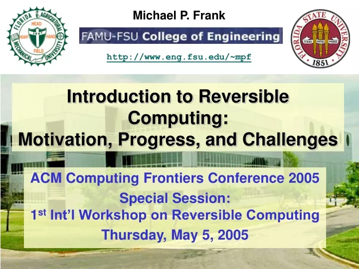
Introduction to Reversible Computing: Motivation, Progress, and Challenges. ACM Computing Frontiers Conference 2005 Special Session: 1 st Int’l Workshop on Reversible Computing Thursday, May 5, 2005. Abstract of Talk.

E N D
Introduction to Reversible Computing: Motivation, Progress, and Challenges ACM Computing Frontiers Conference 2005 Special Session:1st Int’l Workshop on Reversible Computing Thursday, May 5, 2005
Abstract of Talk • The practical performance of a computational process is ultimately limited by its energy efficiency. • Useful work accomplished per unit energy dissipated. • Fundamental physics limits the energy efficiency of conventional, irreversible logic. • The energy efficiency of conventional devices will likely be forced to level off in roughly the next 10-20 years. • Further advances beyond this point will require the use of highly energy-recovering circuit techniques… • and (eventually) this will require an increasing degree of logical reversibility throughout the digital design. • In this talk, we: • explain these motivations for reversible computing, • summarize some recent progress towards its realization • and discuss some outstanding challenges for the field. M. Frank, "Introduction to Reversible Computing"
Introduction to Reversible Computing PART 1: Motivation
Energy Efficiency • The efficiencyη of a process that consumes valued resource R and produces valued product P is the ratio between the amount of product produced, and the amount of resource consumed: η = Pprod/Rcons. • Example 1: A heat engine “consumes” (which in this case, means “degrades”) an amount Q of high-temperature heat energy, and produces an amount W of work. • The heat engine’s efficiency is thus ηh.e. = W/Q. (Dimensionless.) • Of course, ηh.e < 1 because of the conservation of energy… • In the 19th cent., Sadi Carnot showed that ηh.e. ≤ (TH − TL)/TH. • Where TH,TL = temps. of hot, cold thermal reservoirs • Example 2: A computer (i.e., “computational engine”) consumes an amount Econs of free energy, and performs Nops useful computational operations (produces Nops operations worth of useful computational “effort”). • The computer’s (energy) efficiency is thus ηE,comp = Nops/Econs. • Units: Operations per unit energy, or ops/sec/watt. M. Frank, "Introduction to Reversible Computing"
Lower Bounds on Energy Dissipation • In today’s 90 nm VLSI technology, for minimal operations (e.g., conventional switching of a minimum-sized transistor): • Ediss,op is on the order of 1 fJ (femtojoule) ηE≲ 1015 ops/sec/watt. • Will be a bit better in coming technologies (65 nm, maybe 45 nm) • But, conventional digital technologies are subject to several lower bounds on their energy dissipation Ediss,op for digital transitions (logic / storage / communication operations), • And thus, corresponding upper bounds on their energy efficiency. • Some of the known bounds include: • Leakage-based limit for high-performance field-effect transistors: • Maybe roughly ~5 aJ (attojoules) ηE≲ 2×10¹⁷ operations/sec./watt • Reliability-based limit for all non-energy-recovering technologies: • Roughly 1 eV (electron-volt) ηE≲ 6×10¹⁸ ops./sec/watt • von Neumann-Landauer (VNL) bound for all irreversible technologies: • Exactly kT ln 2 ≈ 18 meV ηE≲ 3.5×10²⁰ ops/sec/watt • For systems whose waste heat ultimately winds up in Earth’s atmosphere, • i.e., at temperature T ≈ Troom = 300 K. M. Frank, "Introduction to Reversible Computing"
Trend of Min. Transistor Switching Energy Based on ITRS ’97-03 roadmaps fJ Node numbers(nm DRAM hp) Practical limit for CMOS? aJ Naïve linear extrapolation zJ M. Frank, "Introduction to Reversible Computing"
Reliability Bound on Logic Signal Energies • Let Esig denote the logic signal energy, • The energy involved in storing, transmitting, or transforming a bit’s worth of digital information. • But note that “involved” does not necessarily mean “dissipated!” • As a result of fundamental thermodynamic considerations, it is required that Esig ≥ kBTsig ln R, • Where kB is Boltzmann’s constant, 1.38×10⁻¹² J/K; • and Tsig is the temperature of the local subsystem carrying the signal; • and R is the reliability factor, i.e., the improbability 1/perr of error. • In non-energy-recovering logic technologies (totally dominant today) • Basically all of the signal energy is dissipated to heat on each operation. • And often additional energy (e.g., short-circuit power) as well. • In this case, minimum sustainable dissipation is Ediss,op≳ kBTenv ln R, • Where Tenv is now the temperature of the waste-heat reservoir • Averages around 300 K (room temperature) in Earth’s atmosphere • For a decent R = 2×10¹⁷, this energy is ~40 kT ≈ 1 eV. • For energy efficiency > 1 op/eV, we mustrecover some of the signal energy. • Rather than dissipating it all to heat with each manipulation of the signal. M. Frank, "Introduction to Reversible Computing"
(von Neumann?)-Landauer (VNL) Bound A rigorous result first stated clearly by Rolf Landauer, IBM, 1961 (von Neumann had suggested something similar in 1949 but did not publish details) • Bound is a simple, direct logical consequence of the time-reversibility (invertibility) of all fundamental physical dynamics. • This in turn is implied by the Hamiltonian formulation of all mechanics; e.g., the unitarity of quantum mechanics. Very firmly established! • Invertibility implies physical information can’t be destroyed! • Only reversibly (i.e., mathematically invertibly) transformed! • When we lose or discard a bit’s worth of logical information, • e.g., by erasing or destructively overwriting a bit storage location… • the ‘lost’ information must actually remain in existence, • if not in a known form, then as a bit’s worth (k ln 2) of physical entropy. • Entropy simply means unknown information residing in the physical state. • If the logical bit was originally known (not entropy) • then, entropy has increased in this process by ∆S = 1 bit = k ln 2. • The energy in the heat reservoir must be increased by an amount ∆S·Tenv = kTenv ln 2 in order to accommodate this additional entropy. M. Frank, "Introduction to Reversible Computing"
VNL Bound on Energy Dissipation from Information Loss Follows directly from the reversibility of fundamental physics! N physical microstates per logical macrostatebefore bit erasure(shown as 8 for clarity in this simple example) Physicalmicrostatetrajectories Logical state “0”,after operation S = k ln 8 = 3 bits S = k ln 16 = 4 bits Logical state “0”,before operation ∆S = 1 bit= k ln 2 Logical state “1”,before operation Ediss = ∆S·Tenv = kTenv ln 2 S = k ln 8= 3 bits M. Frank, "Introduction to Reversible Computing"
Reversible Computing • The basic idea is simply this: • Don’t erase information when performing logic / storage / communication operations! • Instead, just reversibly (invertibly) transform it in place! • When reversible digital operations are implemented using well-designed energy-recovering circuitry, • This can result in local energy dissipation Ediss << Esig, • this has already been empirically demonstrated by many groups. • and even total energy dissipation Ediss << kT ln 2! • This has been shown in theory, but we are not yet to the point of demonstrating such low levels of dissipation experimentally. • Achieving this goal requires very careful design, • and verifying it requires very sensitive measurement equipment. M. Frank, "Introduction to Reversible Computing"
Introduction to Reversible Computing PART 2: Progress (1973-2005)
A Few Highlights Of Reversible Computing History • Bennett, 1973-1989: • Reversible Turing machines & emulation algorithms • Can run “virtual” irreversible machines on reversible architectures. • But, the emulation introduces some inefficiencies • Early chemical & Brownian-motion models of physical implementations. • Fredkin and Toffoli, late 1970’s/early 1980’s • Reversible logic gates and networks • Ballistic and adiabatic implementation schemes • Groups @ Caltech,ISI,Amherst,Xerox,MIT, ‘85-’95: • Concepts & implementation for adiabatic circuits in VLSI • Small explosion of adiabatic circuit literature since then • Mid 1990s-today: • Better understanding of overheads, tradeoffs, asymptotic scaling • A few groups begin exploring post-CMOS implementations M. Frank, "Introduction to Reversible Computing"
Early Chemical Implementations • How to physically implement reversible logic? • Bennett’s original inspiration: DNA polymerization! • Reversible copying of a DNA strand • Molecular basis of cell division / organism reproduction • This (and all) chemical reactions are reversible… • Direction (forward vs. backward) & reaction rate depends on relative concentrations of reagent and product species affect free energy • Energy dissipated per step turns out to be proportional to speed. • Implies process is characterized by an energy-time constant. • I call this the “energy coefficient” cE ≡ Ediss,optop = Ediss,op/fop. • For DNA, typical figures are 40 kT ≈ 1eV @ ~1,000 bp/s • Thus, the energy coefficient cE is about 1 eV/kHz. • Can we achieve better energy coefficients? • Yes, in fact, we had already beat DNA’s cE in reversible CMOS VLSI technology circa 1995! M. Frank, "Introduction to Reversible Computing"
Energy Coefficients in Electronics • For a transition involving the adiabatic transfer of an amount Q of charge along a path with resistance R: • The raw (local) energy coefficient is given bycE = Edisst = Pdisst2 = IVt2 = I2Rt2 = Q2R. • Here, V is the voltage drop along the path • Example: In a fairly recent (180 nm) CMOS VLSI technology: • Energy stored per min. sized transistor gate: ~1 fJ @ 2V • Corresponds to charge per gate of Q = 1 fC ≈ 6,000 electrons • Resistance per turned-on transistor of ~14 kΩ • Order of quantum resistance R = R0 = 1/G0 = h/2q2 = 12.9 kΩ • Ideal energy coefficient for a single-gate transition ~1.4×10⁻²⁶ J/Hz • Or in more convenient units, ~80 eV/GHz = 0.08 eV/MHz! • with some expected overheads for a simple test circuit, calculated energy coefficient comes out to about 8× higher, or ~10−25 J·s • Or ~600 eV/GHz = 0.6 eV/MHz. • Detailed Cadence simulations gave us, per transistor: • @ 1 GHz: P = 20 μW, E = 20 fJ = 1.2 keV, so Ec = 1.2 eV/MHz • @ 1 MHz: P = 0.35 pW, E = 3.5 aJ = 2.2 eV, so Ec = 2.1 eV/MHz Q R M. Frank, "Introduction to Reversible Computing"
Simulation Results from Cadence <.01× the power @ 1 MHz >100× faster @ 1 pW/T • Assumptions & caveats: • Assumes ideal trapezoidal power/clock waveform. • Minimum-sized devices, 2λ×3λ* .18 µm (L) × .24 µm (W) • nFET data is shown* pFETs data is very similar • Various body biases tried * Higher Vth suppresses leakage • Room temperature operation. • Interconnect parasitics have not yet been included. • Activity factor (transitions per device-cycle) is 1 for CMOS, 0.5 for 2LAL in this graph. • Hardware overhead from fully- adiabatic design style is not yet reflected * ≥2× transistor-tick hardware overhead in known reversible CMOS design styles 1 nJ 100 pJ Standard CMOS 10 pJ 10 aJ 1 pJ 1 aJ 1 eV Energy dissipated per nFET per cycle 100 fJ 2V 100 zJ 2LAL 1.8-2.0V 1V 10 fJ 10 zJ 0.5V 0.25V 1 fJ kT ln 2 1 zJ 100 aJ 100 yJ M. Frank, "Introduction to Reversible Computing"
A Useful Two-Bit Primitive:Controlled-SET or cSET(a,b) • Semantics: If a=1, then set b:=1. • Conditionally reversible, if the special precondition ab=0 is met. • Note it’s 1-to-1 on the subset of states used • Sufficient to avoid Landauer’s principle • Can implement cSET in dual-rail CMOS with a pair of transmission gates • Each needs just 2 transistors • plus one drive signal • This 2-bit semi-reversible operation & its inverse are together universal for reversible (and irreversible) logic! • If we compose them in special ways. drive (0→1) a switch(T-gate) b b a M. Frank, "Introduction to Reversible Computing"
Reversible OR (rOR) from cSET • Semantics: rOR(a,b) ::= if a|b, c:=1. • Set c:=1 on the condition that either a or b is 1. • Reversible under precondition that initially a|b → ~c. • Two parallel cSETs simultaneouslydriving a single output lineimplements the rOR operation! • This type of composition is not traditionally considered. • Similarly one can do rAND, and reversibleversions of all operations. • Logic synthesis is extremelystraightforward… Hardware diagram a c b Spacetime diagram a’ a a OR b 0 c c’ b’ b M. Frank, "Introduction to Reversible Computing"
O(log n)-time carry-skip adder S A B S A B S A B S A B S A B S A B S A B S A B G Cin GCoutCin GCoutCin G Cin GCoutCin G Cin GCoutCin G Cin P P P P P P P P PmsGlsPls Pms GlsPls PmsGlsPls Pms GlsPls MS MS LS LS G G GCout Cin GCout Cin P P P P Pms GlsPls Pms GlsPls MS LS G GCout Cin P P Pms GlsPls LS GCout Cin P With this structure, we can do a2n-bit add in 2(n+1) logic levels→ 4(n+1) reversible ticks→ n+1 clock cycles. Hardwareoverhead is<2× regularripple-carry! (8 bit segment shown) 3rd carry tick 2nd carry tick 4th carry tick 1st carry tick M. Frank, "Introduction to Reversible Computing"
32-bit Adder Simulation Results 20x better perf.@ 3 nW/adder 1V CMOS 1V CMOS 0.5V CMOS 0.5V CMOS 2V 2LAL, Vsb=1V 2V 2LAL, Vsb=1V (All results normalized to a throughput level of 1 add/cycle) M. Frank, "Introduction to Reversible Computing"
CMOS Gate Implementing rLatch / rUnLatch • Symmetric Reversible Latch Implementation Icon Spacetime Diagram crLatch crUnLatch connect in mem in 2 mem in or connect (in) mem in mem • Just a transmission gate again • This time controlled by a clock, with the data signal driving • Concise, symmetric hardware icon – Just a short orthogonal line • Thin strapping lines denote connection in spacetime diagram. M. Frank, "Introduction to Reversible Computing"
Example: Building cNOT from rlXOR • rlXOR(a,b,c): Reversible latched XOR. • Semantics: c := ab. • Reversible under precondition that c is initially clear. • cNOT(a,b): Controlled-NOT operation. • Semantics: b := ab. (No preconditions.) • A classic “primitive” in reversible & quantum computing • But, it turns out to be fairly complex to implement cNOT in available fully adiabatic hardware… • Thus, it’s really not a very good building block for practical hardware designs! • We can (of course) still build it, if we really want to. • Since, as I said, our gate set is universal for reversible logic M. Frank, "Introduction to Reversible Computing"
cNOT from rlXOR: Hardware Diagram • A logic block providing an in-place cNOT operation (a cNOT “gate”) can be constructed from 2 rlXOR gates and two latched buffers. • The key is: • Operate some of the gates in reverse! Reversiblelatches A B X M. Frank, "Introduction to Reversible Computing"
Introduction to Reversible Computing PART 3: Challenges for the Field
Challenges for the Field • If we want our field to go beyond academia, • and become a practical computing technology, • then we need to address both: • a few remaining technological challenges • and also, a variety of “PR” type challenges • because these are closely coupled! • A convincing technology gets people excited • Positive perceptions more funding, workers M. Frank, "Introduction to Reversible Computing"
Technological Challenges • Fundamental theoretical challenges: • Find more efficient reversible algorithms • Or prove rigorous lower bounds on complexity overheads • Study fundamental physical limits of reversible computing • Implementation challenges: • Design new devices with lower energy coefficients • Design high-quality resonators for driving transitions • Empirically demonstrate large system-level power savings • Application development challenges: • Find a plausible near- to medium-term “killer app” for RC • Something that’s very valuable, and can’t be done without it • Build a prototype RC-based solution prototype M. Frank, "Introduction to Reversible Computing"
Plenty of Room forDevice Improvement Power per device, vs. frequency • Recall, irreversible device technology has at most ~3-4 orders of magnitude of power-performance improvements remaining. • And then, the firm kT ln 2 limit is encountered. • But, a wide variety of proposed reversible device technologies have been analyzed by physicists. • With theoretical power-performance up to 10-12 orders of magnitude better than today’s CMOS! • Ultimate limits are unclear. .18µm CMOS .18µm 2LAL k(300 K) ln 2 Variousreversibledevice proposals M. Frank, "Introduction to Reversible Computing"
(PATENT PENDING, UNIVERSITY OF FLORIDA) MEMS Resonator (One Concept) Moving metal plate support arm/electrode Moving plate Range of Motion Arm anchored to nodal points of fixed-fixed beam flexures,located a little ways away, in both directions (for symmetry) … z y Phase 180° electrode Phase 0° electrode Repeatinterdigitatedstructurearbitrarily manytimes along y axis,all anchored to the same flexure x C(θ) C(θ) 0° 360° 0° 360° θ θ M. Frank, "Introduction to Reversible Computing"
A Challenge for Our Community • I suspect that the field’s critics will never be silenced by theory and simulations alone… • To prove to the world that reversible computing can really work will require a complete empirical demonstration. • We thus cannot afford to continue to sweep issues such as resonator design under the rug… • A convincing demonstration of low total system power must be completely self-contained, including the resonator. • with only DC power input as needed to keep it running • My challenge to us: • Let’s work together to fabricate and empirically demonstrate a simple test chip (e.g., a binary counter) that measurably dissipates much less than the logic signal energy, and eventually much less than some small multiple of kT energy (within a room temperature environment) • Where this measures “wall-plug” power, as our critics like to put it. M. Frank, "Introduction to Reversible Computing"
Public Relations Challenges • Difficulty: Reversible computing is little known • And people have a lot of misconceptions about it. • We need to strive to do better at things like: • Educating the broader science, engineering, and CS community about the field • Including overcoming misconceptions and prejudices • Gaining “political” standing with funding agencies, industry, investors, professional organizations • To lead to the “next level” of more intensive research • Working collaboratively with colleagues in other disciplines (outside CS) who have relevant skills • Device physicists, analog circuit designers, etc. M. Frank, "Introduction to Reversible Computing"
Conclusions • Reversible computing will very likely become necessary within our lifetimes, • if we are to continue progress in computing performance/power. • Much progress in our understanding of RC has been made in the past three decades… • But much important work still remains to be done. • Let’s work together to solve the difficult technological challenges, as well as to raise awareness & improve perceptions of the field. • I hope this workshop will help that to happen M. Frank, "Introduction to Reversible Computing"
Structure of Today’s Session • Sub-session 1: Perspectives on RC (-11:00 am) • Bennett’s keynote, this introductory talk • Eric DeBenedictis on supercomputing apps • Sub-session 2: Novel Impl. Techs. (11:20-12:50) • Sarah Frost, Notre Dame, RC with Quantum Dots • Erik Forsberg, KTH/Zhejiang, Y-branch switches • Sub-session 3: Quasi-reversible circuits (2-3:50) • Four talks, groups from USA, Korea, Germany • Sub-session 4: Rev. comp. theory (4:20-5:20) • Paul Vitanyi, time/space/energy tradeoffs • Levitin & Toffoli, on thermodynamic limits of RC • Panel Discussion: What next steps should we take? M. Frank, "Introduction to Reversible Computing"