Download
1 / 28
280 likes | 314 Views
Understand k-Nearest Neighbor and Naïve Bayes classifiers in machine learning. Learn about distance metrics, neighbor selection, and Bayesian rule derivation. Explore how these algorithms work on real-world data.

E N D
CS 63 Machine Learning:k-Nearest Neighbor, Naïve Bayes, Boosting 18.4, Skim 20.4 Note: These slides require the TeXPPT package (http://users.ecs.soton.ac.uk/srg/softwaretools/presentation/TeX4PPT/)
k-Nearest Neighbor Instance-Based Learning Some material adapted from slides by Andrew Moore, CMU. Visit http://www.autonlab.org/tutorials/ for Andrew’s repository of Data Mining tutorials.
1-Nearest Neighbor • One of the simplest of all machine learning classifiers • Simple idea: label a new point the same as the closest known point Label it red.
1-Nearest Neighbor • A type of instance-based learning • Also known as “memory-based” learning • Forms a Voronoi tessellation of the instance space
Distance Metrics • Different metrics can change the decision surface • Standard Euclidean distance metric: • Two-dimensional: Dist(a,b) = sqrt((a1– b1)2 + (a2– b2)2) • Multivariate: Dist(a,b) = sqrt(∑ (ai– bi)2) Dist(a,b) =(a1 – b1)2 + (a2 – b2)2 Dist(a,b) =(a1 – b1)2 + (3a2 – 3b2)2 Adapted from “Instance-Based Learning” lecture slides by Andrew Moore, CMU.
Four Aspects of anInstance-Based Learner: • A distance metric • How many nearby neighbors to look at? • A weighting function (optional) • How to fit with the local points? Adapted from “Instance-Based Learning” lecture slides by Andrew Moore, CMU.
1-NN’s Four Aspects as anInstance-Based Learner: • A distance metric • Euclidian • How many nearby neighbors to look at? • One • A weighting function (optional) • Unused • How to fit with the local points? • Just predict the same output as the nearest neighbor. Adapted from “Instance-Based Learning” lecture slides by Andrew Moore, CMU.
Zen Gardens Mystery of renowned zen garden revealed [CNN Article] Thursday, September 26, 2002 Posted: 10:11 AM EDT (1411 GMT) LONDON (Reuters) -- For centuries visitors to the renowned Ryoanji Temple garden in Kyoto, Japan have been entranced and mystified by the simple arrangement of rocks. The five sparse clusters on a rectangle of raked gravel are said to be pleasing to the eyes of the hundreds of thousands of tourists who visit the garden each year. Scientists in Japan said on Wednesday they now believe they have discovered its mysterious appeal. "We have uncovered the implicit structure of the Ryoanji garden's visual ground and have shown that it includes an abstract, minimalist depiction of natural scenery," said Gert Van Tonder of Kyoto University. The researchers discovered that the empty space of the garden evokes a hidden image of a branching tree that is sensed by the unconscious mind. "We believe that the unconscious perception of this pattern contributes to the enigmatic appeal of the garden," Van Tonder added. He and his colleagues believe that whoever created the garden during the Muromachi era between 1333-1573 knew exactly what they were doing and placed the rocks around the tree image. By using a concept called medial-axis transformation, the scientists showed that the hidden branched tree converges on the main area from which the garden is viewed. The trunk leads to the prime viewing site in the ancient temple that once overlooked the garden. It is thought that abstract art may have a similar impact. "There is a growing realisation that scientific analysis can reveal unexpected structural features hidden in controversial abstract paintings," Van Tonder said Adapted from “Instance-Based Learning” lecture slides by Andrew Moore, CMU.
k – Nearest Neighbor • Generalizes 1-NN to smooth away noise in the labels • A new point is now assigned the most frequent label of its k nearest neighbors Label it red, when k = 3 Label it blue, when k = 7
k-Nearest Neighbor (k = 9) Appalling behavior! Loses all the detail that 1-nearest neighbor would give. The tails are horrible! A magnificent job of noise smoothing. Three cheers for 9-nearest-neighbor. But the lack of gradients and the jerkiness isn’t good. Fits much less of the noise, captures trends. But still, frankly, pathetic compared with linear regression. Adapted from “Instance-Based Learning” lecture slides by Andrew Moore, CMU.
TheNaïve BayesClassifier Some material adapted from slides by Tom Mitchell, CMU.
The Naïve Bayes Classifier • Recall Bayes rule: • Which is short for: • We can re-write this as:
Deriving Naïve Bayes • Idea: use the training data to directly estimate: • Then, we can use these values to estimate using Bayes rule. • Recall that representing the full joint probability is not practical. and
Deriving Naïve Bayes • However, if we make the assumption that the attributes are independent, estimation is easy! • In other words, we assume all attributes are conditionally independent given Y. • Often this assumption is violated in practice, but more on that later…
Deriving Naïve Bayes • Let and label Y be discrete. • Then, we can estimate and directly from the training data by counting! P(Sky = sunny | Play = yes) = ? P(Humid = high | Play = yes) = ?
The Naïve Bayes Classifier • Now we have: which is just a one-level Bayesian Network • To classify a new point Xnew: Y Labels (hypotheses) j … … Attributes (evidence) X X X 1 i n
The Naïve Bayes Algorithm • For each value yk • Estimate P(Y = yk) from the data. • For each value xij of each attribute Xi • Estimate P(Xi=xij | Y = yk) • Classify a new point via: • In practice, the independence assumption doesn’t often hold true, but Naïve Bayes performs very well despite it.
Naïve Bayes Applications Learning P(BrainActivity | WordCategory) Pairwise Classification Accuracy: 85% People Words Animal Words • Text classification • Which e-mails are spam? • Which e-mails are meeting notices? • Which author wrote a document? • Classifying mental states
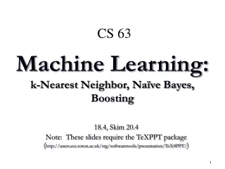
Background: AdaBoost f ( ) g d I N P U T D i i n t t : r a n n g a a x y = i i i 1 ; , = h b f K i i t t t e n u m e r o e r a o n s . ( ) = j j ( ) l f I D D i i i 1 1 t 2 : n a z e w x o r x y = i i i 1 , ; . f K 2 1 t o r : = ; : : : ; + – ( ) d l h h h T X Y D D i i i 3 t t w : r a n m o e : o n w w e g s ! t t h ¯ R C 4 2 : o o s e t . ( ) d h h f l l U D i 5 t t t 2 : p a e e w e g s o r a x y : j j ; 1 ( ) ( ) ( ( ) ) ¯ h ¡ w x w x e x p y x = j j j j 1 t + t t t Z t ( ) h l b d b Z D i i i i t t t w w e r e n o r m a z e s o e a s r u o n 1 t t + . d f 6 e n o r : h h h R i 7 t t t e u r n : e y p o e s s à ! K X ( ) ( ) ¯ h H i x s g n x = t t 1 t = • Classic algorithm by Freund & Schapire (1997) t = 1 – – + + – + + + + – – –
f ( ) g d I N P U T D i i n t t : r a n n g a a x y = i i i 1 ; , = h b f K i i t t t e n u m e r o e r a o n s . ( ) = j j ( ) l f I D D i i i 1 1 t 2 : n a z e w x o r x y = i i i 1 , ; . f K 2 1 t o r : = ; : : : ; + – ( ) d l h h h T X Y D D i i i 3 t t w : r a n m o e : o n w w e g s ! t t h ¯ R C 4 2 : o o s e t . ( ) d h h f l l U D i 5 t t t 2 : p a e e w e g s o r a x y : j j ; 1 ( ) ( ) ( ( ) ) ¯ h ¡ w x w x e x p y x = j j j j 1 t + t t t Z t ( ) h l b d b Z D i i i i t t t w w e r e n o r m a z e s o e a s r u o n 1 t t + . d f 6 e n o r : h h h R i 7 t t t e u r n : e y p o e s s à ! K X ( ) ( ) ¯ h H i x s g n x = t t 1 t = Background: AdaBoost • Classic algorithm by Freund & Schapire (1997) t = 1 – – + + – + + + + – – –
Background: AdaBoost f ( ) g d I N P U T D i i n t t : r a n n g a a x y = i i i 1 ; , = h b f K i i t t t e n u m e r o e r a o n s . ( ) = j j ( ) l f I D D i i i 1 1 t 2 : n a z e w x o r x y = i i i 1 , ; . f K 2 1 t o r : = ; : : : ; + – ( ) d l h h h T X Y D D i i i 3 t t w : r a n m o e : o n w w e g s ! t t h ¯ R C 4 2 : o o s e t . ( ) d h h f l l U D i 5 t t t 2 : p a e e w e g s o r a x y : j j ; 1 ( ) ( ) ( ( ) ) ¯ h ¡ w x w x e x p y x = j j j j 1 t + t t t Z t ( ) h l b d b Z D i i i i t t t w w e r e n o r m a z e s o e a s r u o n 1 t t + . d f 6 e n o r : h h h R i 7 t t t e u r n : e y p o e s s + – Ã ! K X ( ) ( ) ¯ h H i x s g n x = t t 1 t = • Classic algorithm by Freund & Schapire (1997) t = 2 – – + + – + + + + – – –
Background: AdaBoost f ( ) g d I N P U T D i i n t t : r a n n g a a x y = i i i 1 ; , = h b f K i i t t t e n u m e r o e r a o n s . ( ) = j j ( ) l f I D D i i i 1 1 t 2 : n a z e w x o r x y = i i i 1 , ; . f K 2 1 t o r : = ; : : : ; + – ( ) d l h h h T X Y D D i i i 3 t t w : r a n m o e : o n w w e g s ! t t h ¯ R C 4 2 : o o s e t . ( ) d h h f l l U D i 5 t t t 2 : p a e e w e g s o r a x y : j j ; 1 ( ) ( ) ( ( ) ) ¯ h ¡ w x w x e x p y x = j j j j 1 t + t t t Z t ( ) h l b d b Z D i i i i t t t w w e r e n o r m a z e s o e a s r u o n 1 t t + . d f 6 e n o r : h h h R i 7 t t t e u r n : e y p o e s s + – Ã ! K X ( ) ( ) ¯ h H i x s g n x = t t 1 t = • Classic algorithm by Freund & Schapire (1997) t = 2 – – + + – + + + + – – –
Background: AdaBoost f ( ) g d I N P U T D i i n t t : r a n n g a a x y = i i i 1 ; , = h b f K i i t t t e n u m e r o e r a o n s . ( ) = j j ( ) l f I D D i i i 1 1 t 2 : n a z e w x o r x y = i i i 1 , ; . f K 2 1 t o r : = ; : : : ; ( ) d l h h h T X Y D D i i i 3 t t w : r a n m o e : o n w w e g s ! t t h ¯ R C 4 2 : o o s e t . ( ) d h h f l l U D i 5 t t t 2 : p a e e w e g s o r a x y : j j ; 1 ( ) ( ) ( ( ) ) ¯ h ¡ w x w x e x p y x = j j j j 1 t + t t t Z t ( ) h l b d b Z D i i i i t t t w w e r e n o r m a z e s o e a s r u o n 1 t t + . d f 6 e n o r : h h h R i 7 t t t e u r n : e y p o e s s à ! K X ( ) ( ) ¯ h H i x s g n x = t t 1 t = • Classic algorithm by Freund & Schapire (1997) t = 3 – – + + – + + + + – – –
Background: AdaBoost f ( ) g d I N P U T D i i n t t : r a n n g a a x y = i i i 1 ; , = h b f K i i t t t e n u m e r o e r a o n s . ( ) = j j ( ) l f I D D i i i 1 1 t 2 : n a z e w x o r x y = i i i 1 , ; . f K 2 1 t o r : = ; : : : ; ( ) d l h h h T X Y D D i i i 3 t t w : r a n m o e : o n w w e g s ! t t h ¯ R C 4 2 : o o s e t . ( ) d h h f l l U D i 5 t t t 2 : p a e e w e g s o r a x y : j j ; 1 ( ) ( ) ( ( ) ) ¯ h ¡ w x w x e x p y x = j j j j 1 t + t t t Z t ( ) h l b d b Z D i i i i t t t w w e r e n o r m a z e s o e a s r u o n 1 t t + . d f 6 e n o r : h h h R i 7 t t t e u r n : e y p o e s s à ! K X ( ) ( ) ¯ h H i x s g n x = t t 1 t = • Classic algorithm by Freund & Schapire (1997) t = 3 – – + + – + + + + – – –
Background: AdaBoost f ( ) g d I N P U T D i i n t t : r a n n g a a x y = i i i 1 ; , = h b f K i i t t t e n u m e r o e r a o n s . ( ) = j j ( ) l f I D D i i i 1 1 t 2 : n a z e w x o r x y = i i i 1 , ; . f K 2 1 t o r : = ; : : : ; ( ) d l h h h T X Y D D i i i 3 t t w : r a n m o e : o n w w e g s ! t t h ¯ R C 4 2 : o o s e t . ( ) d h h f l l U D i 5 t t t 2 : p a e e w e g s o r a x y : j j ; 1 ( ) ( ) ( ( ) ) ¯ h ¡ w x w x e x p y x = j j j j 1 t + t t t Z t ( ) h l b d b Z D i i i i t t t w w e r e n o r m a z e s o e a s r u o n 1 t t + . d f 6 e n o r : h h h R i 7 t t t e u r n : e y p o e s s à ! K X ( ) ( ) ¯ h H i x s g n x = t t 1 t = • Classic algorithm by Freund & Schapire (1997) t = 4 – – + + – + + + + – – –
Background: AdaBoost f ( ) g d I N P U T D i i n t t : r a n n g a a x y = i i i 1 ; , = h b f K i i t t t e n u m e r o e r a o n s . ( ) = j j ( ) l f I D D i i i 1 1 t 2 : n a z e w x o r x y = i i i 1 , ; . f K 2 1 t o r : = ; : : : ; ( ) d l h h h T X Y D D i i i 3 t t w : r a n m o e : o n w w e g s ! t t h ¯ R C 4 2 : o o s e t . ( ) d h h f l l U D i 5 t t t 2 : p a e e w e g s o r a x y : j j ; 1 ( ) ( ) ( ( ) ) ¯ h ¡ w x w x e x p y x = j j j j 1 t + t t t Z t ( ) h l b d b Z D i i i i t t t w w e r e n o r m a z e s o e a s r u o n 1 t t + . d f 6 e n o r : h h h R i 7 t t t e u r n : e y p o e s s à ! K X ( ) ( ) ¯ h H i x s g n x = t t 1 t = • Classic algorithm by Freund & Schapire (1997) t = 4 – – + + – + + + + – – –
Computing Beta where εt is the training error at time t