Download
1 / 36
380 likes | 577 Views
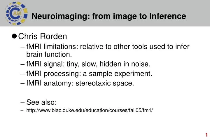
Neuroimaging: from image to Inference. Chris Rorden fMRI limitations: relative to other tools used to infer brain function. fMRI signal: tiny, slow, hidden in noise. fMRI processing: a sample experiment. fMRI anatomy: stereotaxic space. See also:

E N D
Neuroimaging: from image to Inference • Chris Rorden • fMRI limitations: relative to other tools used to infer brain function. • fMRI signal: tiny, slow, hidden in noise. • fMRI processing: a sample experiment. • fMRI anatomy: stereotaxic space. • See also: • http://www.biac.duke.edu/education/courses/fall05/fmri/
Modern neuroscience • Different tools exist for inferring brain function. • No single tool dominates, as each has limitations. • This course focuses on fMRI. poor (whole brain) iap eeg lesions erp nirs pet tms Spatial resolution fmri good (neuron) scr good (millisecond) poor (months) Temporal resolution
Single Cell Recording • Directly measure neural activity. • Exquisite timing information • Precise spatial information • Often, no statistics required! • Each line is one trial. • Each stripe is neuron firing. • Note: firing increases whenever monkey reaches or watches reaching.
Single Cell Recording • With SCR, we are very close to the data. • We can clearly see big effects without processing. • Unfortunately, there are limitations: • Invasive (needle in brain) • Typically constrained to animals, so difficult to directly infer human brain function. • Limited field of view: just a few neurons at a time.
Unlike SCR, we must heavily process fMRI data to extract a signal. The signal in the raw fMRI data is influenced by many factors other than brain activity. We need to filter the data to remove these artifacts. We will examine why each of these steps is used. Processing Steps Motion Correct Spatial Intensity Physiological Noise Removal Temporal Filtering Temporal Slice Time Correct Spatial Smoothing Normalize Statistics fMRI Processing
Unlike SCR, huge delay between activity and signal change. Visual cortex shows peak response ~5s after visual stimuli. Indirect measure of brain activity fMRI signal sluggish 2 1 0 0 6 12 18 24 Time (seconds)
fMRI is ‘Blood Oxygenation Level Dependent’ measure (BOLD). Brain regions become oxygen rich after activity. Very indirect measure. What is the fMRI signal
Anatomical Hypothesis: lesion studies suggest location for motor-hand areas. Ask person to tap finger while in MRI scanner – predict contralateral activity in motor hand area.. Lets conduct a study M1: movement S1: sensation
Task has three conditions: Up arrows: do nothing Left arrows: press left button each time arrow flashes. Right arrows: press right button every time arrow flashes. Block design: each condition repeats rapidly for 11.2 sec. No sequential repeats: block of left arrows always followed by block of either up or right arrows. Task
Participant Lies in scanner watching computer screen. Taps left/right finger after seeing left/right arrows. Collect 120 3D volumes of data, one every 3s (total time = 6min). Data Collection
The scanner reconstructs 120 3D volumes. Each volume = 64x64x36 voxels Each voxel is 3x3x3mm. We need to process this raw data to detect task-related changes. Raw Data
Unfortunately, people move their heads a little during scanning. We need to process the data to create motion-stabilized images. Otherwise, we will not be looking at the same brain area over time. Motion Correction
Each voxel is noisy By blurring the image, we can get a more stable signal (neighbors show similar effects, noise spikes attenuated). Spatial smoothing
We need to generate a statistical model. We convolve expected brain activity with hemodynamic response to get predicted signal. Predicted fMRI signal Neural Signal HRF Predicted fMRI signal =
We generate predictions for neural responses for the left and right arrows across our dataset. Statistics will identify which areas show this pattern of activity. Several possible statistical contrasts (crucial to inference): Activity correlated with left arrows: visual cortex, bilateral motor. More activity for left than right arrows: contralateral motor. Predicted fMRI signal
Voxelwise statistics • We compute the probability for every voxel in the brain. • We observe that right arrows precede activation in the left motor cortex and right cerebellum.
Right motor cortex becomes brighter following movement of left hand. Note signal increases from ~12950 to ~13100, only about 1.2% And this is after all of our complicated processing to reduce noise. fMRI signal change is tiny, noise is high
Coordinates - normalization • Different people’s brains look different • ‘Normalizing’ adjusts overall size and orientation Normalized Images Raw Images
Why normalize? • Stereotaxic coordinates analogous to longitude • Universal description for anatomical location • Allows other to replicate findings • Allows between-subject analysis: crucial for inference that effects generalize across humanity.
Goals for this course • fMRI is notoriously difficult technique • Sluggish signal • Poor signal/noise • Must find meaningful statistical contrasts • This seminar reveals how to • Devise meaningful contrasts • Maximize signal, minimize noise • Control for statistical errors.
Safety • MRI uses very strong magnet and radiofrequencies • 3T= ~x60,000 field that aligns compass • Metal and electronic devices are not compatible. • MRI scanning makes loud sounds • Rapid gradient switching creates auditory noise. • Auditory protection crucial. • MRI scanning is confined • Claustrophobia is a concern.
Summary of Lectures • Introduction • Physics I: Hardware and Acquisition • Physics II: Contrasts and Protocols • fMRI Paradigm Design • fMRI Statistics and Thresholding • fMRI Spatial Processing • fMRI Temporal Processing • VBM & DTI: subtle structural changes • Lesion Mapping: overt structural changes • Advanced and Alternative Techniques
Which tools • There are many tools available for analysis. • Different strengths. • We predominantly focus on SPM and FSL. • These are both free, popular and have good user support. https://cirl.berkeley.edu/view/Grants/BrainPyMotivation
Reporting findings • How do we describe anatomy to others? • We could use anatomical names, but often hard to identify. • We could use Brodmann’s Areas, but this requires histology – not suitable for invivo research. • Both show large between-subject variability. • Requires anatomical coordinate system.
Relative Coordinates • On the globe we talk about North, South, East and West. • Lets explore the coordinates for the brain.
Orientation - animals • Cranialhead • Rostralbeak • Dorsalback Dorsal Rostral Caudal Ventral • Caudaltail • Ventralbelly
Coordinates – Dorsal Ventral • Human dorsal/ventral differ for brain and spine. • Head/Foot, Superior/Inferior, Anterior/Posterior not ambiguous. Dorsal Ventral Dorsal Ventral Dorsal Ventral
Coordinates – Human • Human rostral/caudal differ for brain and spine. • Head/Foot, Superior/Inferior, Anterior/Posterior not ambiguous. C R R R C C
Orientation • Human anatomy described as if person is standing • If person is lying down, we would still say the head is superior to feet.
Anatomy – Relative Directions lateral < medial > lateral Posterior <> Anterior Ventral/Dorsal aka Inferior/Superior aka Foot/Head Ventral <> Dorsal Anterior/Posterior aka Rostral/Caudal Posterior <> Anterior
coronal sagittal axial Coordinates - Anatomy • 3 Common Views of Brain: • Coronal (head on) • Axial (bird’s eye), aka Transverse. • Sagittal (profile)
Coronal • Corona: a coronal plane is parallel to crown that passes from ear to ear
Transverse • Transverse/Axial: perpendicular to the long axis Example: cucumber slices are transverse to long axis.
Sagittal • Sagittal – ‘arrow like’ • Sagittal cut divides object into left and right • sagittal suture looks like an arrow. top view
Sagittal and Midsagittal • A Sagittal slice down the midline is called the ‘midsagittal’ view. midsagittal sagittal
Oblique Slices • Slices that are not cut parallel to an orthogonal plane are called ‘oblique’. • The oblique blue slice is neither Coronal nor Axial. Cor Oblique Ax