Download
1 / 49
500 likes | 597 Views
GENERAL LINEAR MODELS: Estimation algorithms. KIM MINKALIS. GOAL OF THE THESIS. THE GENERAL LINEAR MODEL. The general linear model is a statistical linear model that can be written as: . where: Y is a matrix with series of multivariate measurements

E N D
GENERAL LINEAR MODELS:Estimation algorithms KIM MINKALIS
THE GENERAL LINEAR MODEL The general linear model is a statistical linear model that can be written as: where: Y is a matrix with series of multivariate measurements X is a matrix that might be a design matrix B is a matrix containing parameters that are usually to be estimated U is a matrix containing errors or noise The residual is usually assumed to follow a multivariate normal distribution. The general linear model incorporates a number of different statistical models: ANOVA, ANCOVA, MANOVA, MANCOVA, ordinary linear regression, t-test and F-test. If there is only one column in Y (i.e., one dependent variable) then the model can also be referred to as the multiple regression model (multiple linear regression).
SIMPLE LINEAR REGRESSION Simple Linear Model in Scalar Form: Consider now writing an equation for each observation: Simple Linear Model in Matrix Form: • X is called the design matrix • βis the vector of parameters • εis the error vector • Y is the response vector
SIMPLE LINEAR REGRESSION Distributional Assumptions in Matrix Form
SIMPLE LINEAR REGRESSION Least squares ALTERNATE METHODS: MLE REML GEE
SUMS OF SQUARES TOTAL SUM OF SQUARES = RESIDUAL (ERROR) SUM OF SQUARES + EXPLAINED (MODEL) SUM OF SQUARES SST SSE SSR SST is the sum of the squares of the difference of the dependent variable and its grand mean (total variation in Y – outcome variable) SSR is the sum of the squares of the differences of the predicted values and the grand mean (variation explained by the fitted model) SSE is a measure of the discrepancy between the data and an estimation model (unexplained residual variation)
SUMS OF SQUARES and mean squares The sums of squares for the analysis of variance in matrix notation is: Degrees of freedom Mean squares
Example 1 simple linear regression DATA To read from an existing SAS dataset, submit a USE command to open it. The general form of the USE statement is: USE sas dataset <VAR operand> <WHERE expression>; Transferring data from a SAS data set to a matrix is done with the READ statement. READ <range> <var operand> <where expression> <into name> ; READING DATA INTO IML
Example 1 simple linear regression Number of observations 15 Number of parameters for fixed effects 2 Vector of estimated regression coefficients Degrees of Freedom 15-2=13 Variance-Covariance Matrix for Beta Standard Error of Beta (2X1 vector)
Example 1 simple linear regression A/B means DIVIDE COMPONENTWISE (A and B must be the same size) t-statistics for tests of significant regression coefficients Probf(A,d1,d2) is Prob[F(d1,d2) ≤ A] for an F distribution Recall T(d)2 = F(1,d), so that 1-Probf(T#T,1,d) returns two-sided Student-t P-values SST SSR MSR
Example 1 simple linear regression PROC GLM PROC iml EXAMPLE
MULTIPLE LINEAR REGRESSION MODEL MATRIX ALGEBRA IS EXACTLY THE SAME!
Example 2 SINGLE FACTOR ANALYSIS OF VARIANCE DATA Dataset has a total of 19 observations (Store-Design Combinations) Cases (Outcome Variable) = Number of cases sold Design = 1 of 4 different package designs for new breakfast cereal Store = 5 stores with approximately same sales volume Need to create multiple columns to represent levels within categorical factor USE PROC IML USE DATA STEP
Example 2 SINGLE FACTOR ANALYSIS OF VARIANCE The DESIGN function creates a design matrix of 0s and 1s from column-vector. Each unique value of the vector generates a column of the design matrix. This column contains ones in elements with corresponding elements in the vector that are the current value; it contains zeros elsewhere. The DESIGNF function works similar to the DESIGN function; however, the result matrix is one column smaller and can be used to produce full-rank design matrices. The result of the DESIGNF function is the same as if you took the last column off the DESIGN function result and subtracted it from the other columns of the result. DESIGN FUNCTION DESIGNF FUNCTION DATA STEP
Example 2 SINGLE FACTOR ANALYSIS OF VARIANCE MATRIX A Generalized Inverse Note that column 5 can be written as a linear column 1 − column 2 − column 3 − column 4 Matrix does not have a unique inverse conditional Inverse pseudo Inverse Same mathematics as multiple linear regression model Constructing the design matrix is the only trick MATRIX G AG AGA=A
Example 2 SINGLE FACTOR ANALYSIS OF VARIANCE PROC GLM PROC iml EXAMPLE
Analysis OF COVARIANCE (ANCOVA) ANOVA+Regression Categorical+Continuous ANCOVA is used to account/adjust for Pre-Existing Conditions In our example we will model the Area Under the Curve per Week is adjusted for the Baseline Beck Depression Score Index (Continuous), the Gender of the Subject (Categorical) and the Type of Treatment (Categorical). Some models may only have one covariate representing the baseline score and the outcome variable represents the final score – it may be tempting to get rid of the covariate by modeling the difference. This may be problematic as you are forcing a slope of 1. We also have to make use of partial F tests to compare two models. EXAMPLE
CONSTRUCTION OF LEAST SQUARE MEANS In PROC GLM what is the difference between the MEANS and the LSMEANS statement? When the MEANS statement is used, PROC GLM computes the arithmetic means (average) of all continuous variables in the model (both dependent and independent) for each level of the categorical variable specified in the MEANS statement. When the LSMEANS statement is used, PROC GLM computes the predicted population margins; that is, they estimate marginal means over a balanced population. Means corrected for imbalances in other variables. When an experiment is balanced, MEANS and LSMEANS agree. When data are unbalanced, however, there can be a large difference between a MEAN and an LSMEAN.
CONSTRUCTION OF LEAST SQUARE MEANS Assume A has 3 levels, B has 2 levels, and C has 2 levels, and assume that every combination of levels of A and B exists in the data. Assume also that Z is a continuous variable with an average of 12.5. Then the least-squares means are computed by the following linear combinations of the parameter estimates:
Example LSMEANS PROC GLM PROC iml EXAMPLE
MAXIMUM LIKELIHOOD ESTIMATION With linear models it is possible to derive estimators that are optimal in some sense As models become more general optimal estimators become more difficult obtain and estimators that are asymptotically optimal are obtained instead Maximum likelihood estimators (MLE) have a number of nice asymptotic properties and are relatively easy to obtain Start with the distribution of our data:
MAXIMUM LIKELIHOOD ESTIMATION HESSIAN GRADIENT GRADIENT INFORMATION MATRIX Regardless of the algorithm used the MLE of the model parameters remain the same:
MAXIMUM LIKELIHOOD ESTIMATION VERSUS Ordinary least squares FIXED EFFECTS estimation Independence of Mean and Variance for Normals Independence of Estimators Variance estimation OLS is an unbiased estimator ML is a biased estimator Note that the ML formula differs from the OLS formula by dividing by N and not N-p
ITERATIVE METHODS NEWTON RAPHSON METHOD OF SCORING
EXTENSION OF THE GENERAL LINEAR MODEL In a linear model it is assumed that there is a single source of variability. One can extend linear models by allowing for multiple sources of variability. In the simplest case, the combined covariance matrix is a linear function of the variance components. In other cases, the combined covariance matrix is a non-linear function of the variance components. The linear form is typical of the structure encountered in various split plot designs and the non-linear form is typical of repeated measure designs. MIXED LINEAR MODEL EQUATION
MIXED LINEAR MODELS Set derivative equal to zero and solve for β: Plug β into derivatives with respect to σi2
MIXED LINEAR MODELS Maximum Likelihood solutions equating derivatives equal to zero: Fixed Effects Variance components We can make an algebraically simpler expression for the second equation by defining P in the following manner: Note that sesq(M) represents the sum of squares of elements of M
MIXED LINEAR MODELS Second Partials
MIXED LINEAR MODELS FISHER SCORING – EXPECTED VALUES
RESTRICTED (Residual )MAXIMUM LIKELIHOOD (REML) Maximum Likelihood does not yield the usual estimators when the data are balanced In estimating variance components ML does not take into account the degrees of freedom that are involved in estimating fixed effects Estimating variance components based on residuals calculated after fitting by ordinary least squares just the fixed effects part of the model
MIXED EFFECTS Example Actual levels of milk fat in its yogurt exceeded the labeled amount Outcome Variable = Fat Content of each Yogurt Sample (3.0) Random Effect = 4 Randomly Chosen Laboratories Fixed Effect = Government’s VS Sheffield’s Method 6 samples where sent to each laboratory but Government’s Labs had technical difficulties and were not able to determine fat content for all 6 samples.
MIXED EFFECTS Example The GLMMOD procedure constructs the design matrix for a general linear model; it essentially constitutes the model-building front end for the GLM procedure. PROC GLMMOD
MIXED EFFECTS Example PARTIAL DATA
MIXED EFFECTS Example Z Matrix G Matrix R Matrix ZGZ’ Matrix ZGZ’+R Matrix
MIXED EFFECTS Example READ DATA INTO PROC IML RANDOM EFFECTS Recall that columns 2-5 represent the 4 different labs and columns 6-13 represent the interaction between labs and methods Need to get rid of column 1 which represents the intercept FIXED EFFECTS Recall that column 1 represents the intercept and columns 2 and 3 represent the two different methods The outcome variable fat is read into the vector y
MIXED EFFECTS Example Get initial estimates for variance components Use MSE from model containing only fixed effects as initial estimate Note: We used biased estimate from ML approach 0.1113189 (ML) instead of 0.11733610 (OLS) for initial estimates G is aq x q matrix where q is the number of random effect parameters. G is always diagonal in a random effects model if the random effects are assumed uncorrelated. In our example, starting value for G is a 12X12 diagonal matrix G0 = 0.0556594* I(12) R0 = 0.0556594 *I(39)
MIXED EFFECTS Example LOG LIKELIHOOD GRADIENT RESIDUAL NOTE: W represents a 39X4 design matrix representing levels of factor LAB S represents a 39X8 design matrix representing the levels of the Interaction between LAB*METHOD
MIXED EFFECTS Example HESSIAN NOT POSITIVE DEFINITE ADD 215 TO MAIN DIAGONAL
MIXED EFFECTS EXAmPLE CALL NLPNRR USER DEFINED FUNCTIONS AND CALL ROUTINES
MIXED EFFECTS EXAMPLE HESSIAN Use PROC IML Nonlinear Optimization and Related Subroutines
MIXED EFFECTS Example Variance Components must be positive Hessian must be positive definite Use CALL NLPNRR EXAMPLE
MIXED EFFECTS Example 215 = 32768 214 = 16384 212 = 4096 28 = 256 26 = 64 24 = 16 22 = 4
MIXED EFFECTS Example Variance Components PROC IML PROC MIXED