Download
1 / 16
170 likes | 252 Views
Learning in the BPN. Gradients of two-dimensional functions:.

E N D
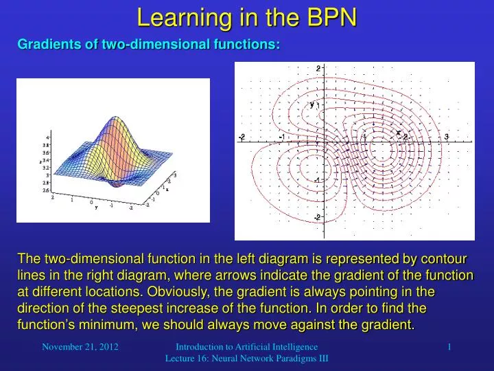
Learning in the BPN • Gradients of two-dimensional functions: The two-dimensional function in the left diagram is represented by contour lines in the right diagram, where arrows indicate the gradient of the function at different locations. Obviously, the gradient is always pointing in the direction of the steepest increase of the function. In order to find the function’s minimum, we should always move against the gradient. Introduction to Artificial Intelligence Lecture 16: Neural Network Paradigms III
Learning in the BPN • In the BPN, learning is performed as follows: • Randomly select a vector pair (xp, yp) from the training set and call it (x, y). • Use x as input to the BPN and successively compute the outputs of all neurons in the network (bottom-up) until you get the network output o. • Compute the error opk, for the pattern p across all K output layer units by using the formula: Introduction to Artificial Intelligence Lecture 16: Neural Network Paradigms III
Learning in the BPN • Compute the error hpj, for all J hidden layer units by using the formula: • Update the connection-weight values to the hidden layer by using the following equation: Introduction to Artificial Intelligence Lecture 16: Neural Network Paradigms III
Learning in the BPN • Update the connection-weight values to the output layer by using the following equation: • Repeat steps 1 to 6 for all vector pairs in the training set; this is called a training epoch. • Run as many epochs as required to reduce the network error E to fall below a threshold : Introduction to Artificial Intelligence Lecture 16: Neural Network Paradigms III
fi(neti(t)) = 0.1 1 = 1 0 neti(t) -1 1 Sigmoidal Neurons • In backpropagation networks, we typically choose = 1 and = 0. Introduction to Artificial Intelligence Lecture 16: Neural Network Paradigms III
Sigmoidal Neurons • In order to derive a more efficient and straightforward learning algorithm, let us use a simplified form of the sigmoid function. We do not need a modifiable threshold ;instead, let us set = 0 and add an offset (“dummy”) input for each neuron that always provides an input value of 1. Then modifying the weight for the offset input will work just like varying the threshold. The choice = 1 works well in most situations and results in a very simple derivative of S(net): Introduction to Artificial Intelligence Lecture 16: Neural Network Paradigms III
Sigmoidal Neurons Very simple and efficient to compute! Introduction to Artificial Intelligence Lecture 16: Neural Network Paradigms III
Learning in the BPN Then the derivative of our sigmoid function, for example, f’(netk) for the output neurons, is: Introduction to Artificial Intelligence Lecture 16: Neural Network Paradigms III
Learning in the BPN • Now our BPN is ready to go! • If we choose the type and number of neurons in our network appropriately, after training the network should show the following behavior: • If we input any of the training vectors, the network should yield the expected output vector (with some margin of error). • If we input a vector that the network has never “seen” before, it should be able to generalize and yield a plausible output vector based on its knowledge about similar input vectors. Introduction to Artificial Intelligence Lecture 16: Neural Network Paradigms III
Backpropagation Network Variants • The standard BPN network is well-suited for learning static functions, that is, functions whose output depends only on the current input. • For many applications, however, we need functions whose output changes depending on previous inputs (for example, think of a deterministic finite automaton). • Obviously, pure feedforward networks are unable to achieve such a computation. • Only recurrent neural networks (RNNs) can overcome this problem. • A well-known recurrent version of the BPN is the Elman Network. Introduction to Artificial Intelligence Lecture 16: Neural Network Paradigms III
The Elman Network • In comparison to the BPN, the Elman Network has an extra set of input units, so-called context units. • These neurons do not receive input from outside the network, but from the network’s hidden layer in a one-to-one fashion. • Basically, the context units contain a copy of the network’s internal state at the previous time step. • The context units feed into the hidden layer just like the other input units do, so the network is able to compute a function that not only depends on the current input, but also on the network’s internal state(which is determined by previous inputs). Introduction to Artificial Intelligence Lecture 16: Neural Network Paradigms III
The Elman Network Introduction to Artificial Intelligence Lecture 16: Neural Network Paradigms III
The Counterpropagation Network • Another variant of the BPN is the counterpropagation network (CPN). • Although this network uses linear neurons, it can learn nonlinear functions by means of a hidden layer of competitive units. • Moreover, the network is able to learn a function and its inverse at the same time. • However, to simplify things, we will only consider the feedforward mechanism of the CPN. Introduction to Artificial Intelligence Lecture 16: Neural Network Paradigms III
Output layer Y1 Y2 Hiddenlayer H1 H2 H3 Input layer X1 X2 The Counterpropagation Network • A simple CPN network with two input neurons, three hidden neurons, and two output neurons can be described as follows: Introduction to Artificial Intelligence Lecture 16: Neural Network Paradigms III
The Counterpropagation Network • The CPN learning process (general form for n input units and m output units): • Randomly select a vector pair (x, y) from the training set. • Normalize (shrink/expand to “length” 1) the input vector x by dividing every component of x by the magnitude ||x||, where Introduction to Artificial Intelligence Lecture 16: Neural Network Paradigms III
The Counterpropagation Network • Initialize the input neurons with the normalized vector and compute the activation of the linear hidden-layer units. • In the hidden (competitive) layer, determine the unit W with the largest activation (the winner). • Adjust the connection weights between W and all N input-layer units according to the formula: • Repeat steps 1 to 5 until all training patterns have been processed once. Introduction to Artificial Intelligence Lecture 16: Neural Network Paradigms III