Download

1 / 18
210 likes | 378 Views
Properties of Demand Functions. Comparative statics analysis of ordinary demand functions -- the study of how ordinary demands x 1 *(p 1 ,p 2 ,m) and x 2 *(p 1 ,p 2 ,m) change as prices p 1 , p 2 and income m change. Own-Price changes:

E N D
Properties of Demand Functions • Comparative statics analysis of ordinary demand functions -- the study of how ordinary demands x1*(p1,p2,m) and x2*(p1,p2,m) change as prices p1, p2 and income m change. • Own-Price changes: • How does x1*(p1,p2,m) change as p1 changes, holding p2 and m constant?
p1 Own-Price Changes Ordinarydemand curvefor commodity 1 Fixed p2 and m. p1’’’ p1’’ p1’ x1* x1*(p1’) x1*(p1’’’) x1*(p1’’) x1*(p1’’’) x1*(p1’) x1*(p1’’)
Own-Price Changes • The curve containing all the utility-maximizing bundles traced out as p1 changes, with p2 and m constant, is the p1- price offer curve. • The plot of the x1-coordinate of the p1- price offer curve against p1 is the ordinary demand curve for commodity 1.
Own-Price Changes: Cobb-Douglas • Take • Then the ordinary demand functions for commodities 1 and 2 are • What does the demand curve look like? • What does a p1 price-offer curve look like?
p1 Own-Price Changes Ordinarydemand curvefor commodity 1 is Fixed p2 and m. x1* x1*(p1’’’) x1*(p1’) x1*(p1’’)
Own-Price Changes: Perfect complements • Take • Then the ordinary demand functionsfor commodities 1 and 2 are • What does the demand curve look like? • What is the p1 price-offer curve?
p1 Own-Price Changes Ordinarydemand curvefor commodity 1 is Fixed p2 and m. p1’’’ x2 p1’’ m/p2 p1’ x1* x1
Own-Price Changes: Perfect Substitutes • Take • Then the ordinary demand functionsfor commodities 1 and 2 are • What does the demand curve look like? • What is the p1 price-offer curve?
p1 Own-Price Changes Ordinarydemand curvefor commodity 1 Fixed p2 and m. p1’’’ x2 p2 = p1’’ p1 price offer curve p1’ x1* x1
Income Changes • How does the value of x1*(p1,p2,m) change as m changes, holding both p1 and p2 constant? • A plot of quantity demanded against income is called an Engel curve. • A plot of bundles chosen as we vary income is called the income-offer curve. • Draw these two curves for Perfect complements, Cobb-Douglas, and Perfect Substitutes.
Income Changes • In every example so far the income offer curves have all been straight lines for the origin?Q: Is this true in general? • A: No. Income offer curves are straight lines only if the consumer’s preferences are homothetic.
Homotheticity • A consumer’s preferences are homothetic if and only iffor every k > 0. • That is, the consumer’s MRS is the same anywhere on a straight line drawn from the origin. p p Û (x1,x2) (y1,y2) (kx1,kx2) (ky1,ky2)
Why the connection? • Take a budget and choice (x1*,x2*). Double the budget so new budget is 2m. • Notice if (x1,x2) were in the old budget, (2 x1, 2 x2) is in the new budget. • Homotheticity implies that if (x1*,x2*)> (x1,x2) then (2x1*,2x2*)>(2x1,2x2), thus new choice is (2x1*,2x2*). • Notice if you draw a line from origin to (x1*,x2*) it goes through (2x1*,2x2*). • Since these are the choices, the MRS must be the same at both points to be tangent to the ICs.
Homogeneous Utility Functions • U(k x1,k x2)= g(k) u(x1,x2) and g(k)>0. • This implies homotheticity! • U(x1,x2)>U(y1,y2) => g(k) U(x1,x2)> g(k) U(y1,y2) => U(k x1,k x2)>U(k y1,k y2) • Does Cobb-Douglas, Perfect Substitutes, Perfect Complements satisfy this?
Income Effects -- A Nonhomothetic Example • Quasilinear preferences are not homothetic. • For example, • U(1,0)>U(0,3/4) but when k=4, we have U(4,0)<U(0,3)!
Income Effects • A good for which quantity demanded rises with income is called normal. • Therefore a normal good’s Engel curve is positively sloped. • A good for which quantity demanded falls as income increases is called income inferior. • Therefore an income inferior good’s Engel curve is negatively sloped. • A luxury good is where the proportion of income spent on it goes up with income. • The opposite of a luxury good is a necessarygood. • Is a necessary good always inferior? • Is a inferior good always necessary? • Can we have a necessary good w/o a luxury good? Vice-versa? • Can we have an inferior good w/o a luxury good? Vice-versa?
Ordinary and Giffen goods. • A good is called ordinary if the quantity demanded of it always increases as its own price decreases. • If, for some values of its own price, the quantity demanded of a good rises as its own-price increases then the good is called Giffen. • Example of a Giffen good – U(x1,x2)=-e-x1-e-x2
Cross-Price Effects • If an increase in p2 • increases demand for commodity 1 then commodity 1 is a gross substitute for commodity 2. • reduces demand for commodity 1 then commodity 1 is a gross complement for commodity 2. • What happens with Cobb-Douglas preferences?